In earlier discussions, the set ℝ ^m appeared in a variety of contexts: as a vector space (also denoted by ℝ ^m ), an inner product space (ℝ ^m , ), a normed vector space (ℝ ^m , ||·||), a metric space (ℝ ^m , ), and a topological space (ℝ ^m , ). Section 9.4 outlines the logical connections between these spaces. Looking back at Chapter 10, it would have been more precise, although cumbersome, to use the notation (ℝ ^m , , ||·||, , ), or at least (ℝ ^m , ), instead of simply ℝ ^m when discussing Euclidean derivatives and integrals. In this chapter, we are concerned with many of the same concepts considered in Chapter 10, but this time exclusively for M = 3. We use the notation ℝ³ in the preceding generic manner, allowing the structures relevant to a particular discussion to be left implicit. Aside from notational convenience, this has the added virtue of reserving the notation and later for more specific purposes in Chapter 12.

11.1 Curves inℝ³

Recall from Section 10.1 the definition of a (parametrized) curve in ℝ³ and what it means for such a curve to be smooth. A smooth curve λ(t) : (a, b) → ℝ³ is said to be regular if its velocity (dλ/dt)(t) : (a, b) → ℝ³ is nowhere‐vanishing. Let g(u) : (c, d) → (a, b) be a diffeomorphism. Since λ and g are smooth, by Theorem 10.1.12, so is λ ∘ g. We say that the curve λ ∘ g(u) : (c, d) → ℝ³ is a smooth reparametrization of λ .

Theorem 11.1.1 can be used to define an equivalence relation on the collection of smooth curves as follows: for two such curves λ and ψ, we write λ ~ ψ φ if φ is a smooth reparametrization of λ. This idea will not be pursued further, but it makes the point that our focus should be on the intrinsic properties of a “curve”, for example, whether it is regular, and not the specifics of a particular parametrization.

11.2 Regular Surfaces inℝ³

Our immediate goal in this section is to define what we temporarily refer to as a “smooth surface”. We all have an intuitive idea of what it means for a geometric object to be “smooth”. For example, the sphere definitely has this property, but not the cube. The challenge is to translate such intuition into rigorous mathematical language. A feature of the sphere that gives it “smoothness” is our ability to attach to each of its points a unique “tangent plane”, something that is not possible for the cube.

Let U be an open set in ℝ² , and let φ: U → ℝ³ be a smooth map. In the present context, we refer to φ as a parametrized surface. The differential map at a point q in U is d _q (φ): ℝ² → ℝ³ . It follows from Theorem 10.2.1 that if φ is an immersion at q, then d _q (φ)(ℝ² ) is a 2‐dimensional vector space, which we can view as a “tangent plane” to the graph of φ at φ (q). This suggests that a “smooth surface” might reasonably be defined to be the image of a parametrized surface when the latter has the added feature of being an immersion. Before exploring this concept, we need to establish the notation for coordinates in ℝ² and ℝ³ .

In this chapter and the next, coordinates on ℝ² are denoted by (r ¹ , r ² ) or (r, s), and those on ℝ³ by (x ¹ , x ² , x ³ ) or (x, y, z).

We sometimes, especially in the examples, identify ℝ² with the xy‐plane in ℝ³ . In that setting, coordinates on ℝ² are denoted by (x, y).

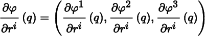
Let U be an open set in ℝ² , and let φ = (φ ¹, φ ², φ ³) : U → ℝ³ be a parametrized surface. Since φ is smooth, by definition, so are φ ¹, φ ², and φ ³. For each q in U, we have

hence

(11.2.1)

for i = 1, 2. For brevity, let us denote

The vector product approach in part (e) of Theorem 11.2.2 is a computationally convenient way of determining whether a parametrized surface is an immersion, and we will use it often.

For simplicity, the figures for the next two examples have been drawn in the xy‐plane of ℝ³ , leaving it to the reader to imagine the suppressed z‐axis.

The upshot of the preceding examples is that φ being an immersion is necessary for φ(U) to be “smooth”, but not sufficient. At a minimum, we need to add the requirement that φ (U) does not self‐intersect, or equivalently, that φ is injective. Further examples (that will not be presented) reveal additional deficiencies inherent in defining a “smooth surface” to be the image of some type of parametrized surface.

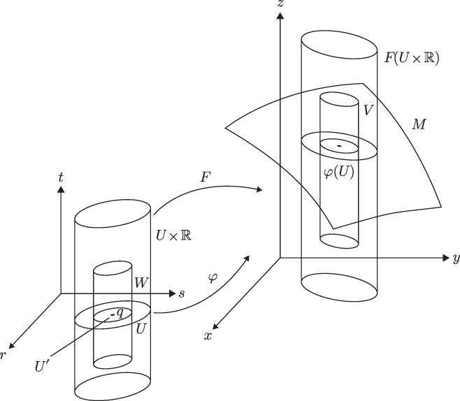
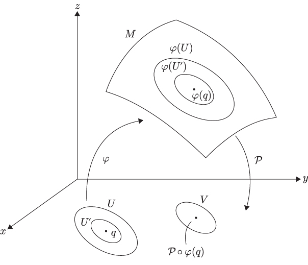
We now take a different approach to the problem that can be loosely described as follows: a “smooth surface” is defined to be a topological subspace of ℝ³ that can be covered in a piecewise fashion by a collection of parametrized surfaces in such a way that the pieces “fit together nicely”. We need to make all this precise.

Let M be a topological subspace of ℝ³ . A chart (on M) is a pair (U, φ), where U is an open set in ℝ² and φ : U → ℝ³ is a parametrized surface such that:

[C1] φ : U → ℝ³ is an immersion.

[C2] φ (U) is an open set in M.

[C3] φ : U → φ (U) is a homeomorphism.

Condition [C1] has been discussed in detail. Conditions [C2] and [C3] are far from intuitive, but we can at least say about [C3] that it ensures φ is injective, thereby avoiding the problem of self‐intersection discussed above.

When it is necessary to make the components of φ explicit in (U, φ), we use the notation (U, φ = (φ ⁱ )) or (U, φ = (φ ¹, φ ², φ ³)). We refer to U as the coordinate domain of the chart, and to φ as its coordinate map. For each point p in φ (U), (U, φ) is said to be a chart at p . When φ (U) = M, we say that (U, φ) is a covering chart on M, and that M is covered by (U, φ). Two charts, (U, φ) and on M are said to be overlapping if is nonempty. In that case, the map

is called a transition map. For brevity, we usually denote

An atlas for M is a collection of charts on M such that the φ _α (U _α ) form an open cover of M; that is,

We are now in a position to replace our preliminary attempt at describing a “smooth surface” with something definitive. A regular surface (in ℝ³ ) is a pair (M, ), where M is a topological subspace of ℝ³ and is an atlas for M. A noteworthy feature of this definition is that it places no requirements on the choice of charts making up the atlas other than that their coordinate domains cover M. We usually adopt the shorthand of referring to M as a regular surface, with understood from the context.

Throughout, any chart on a regular surface is viewed as a regular surface.

An implication of Theorem 11.2.7 is that in order to investigate whether a function or map that has a regular surface as its domain is smooth, we need to rely on the extended version of smoothness described at the end of Section 10.1. The next result is an important case in point.

By definition, a regular surface is a patchwork of images of parametrized surfaces. The next result shows that instead of images of parametrized surfaces, we can use graphs of smooth functions.

Theorem 11.2.12 shows that the existence of charts on regular surfaces makes it possible to answer questions about extended smoothness of maps on regular surfaces using methods developed for Euclidean smoothness.

We close this section with an example of a chart on the unit sphere that is strikingly different from the charts constructed in Example 11.2.6.

11.3 Tangent Planes inℝ³

Having defined a regular surface and established some of its basic properties, we are now in a position to present a rigorous definition of “tangent plane”.

Let M be a regular surface. A curve (on M) is a curve λ(t): I → M as defined in Section 11.1, with the additional feature that it takes values in M. Let p be a point in M. We say that a vector V in ℝ³ is a tangent vector to M at p if there is a smooth curve λ(t): (a, b) → M such that λ(t ₀) = p and (dλ/dt)(t ₀) = v for some t ₀ in (a, b). The tangent plane of M at p is denoted by T _p (M) and defined to be the set of all such tangent vectors:

In the notation of Theorem 11.3.1, let us denote

and

We refer to ℋ as the coordinate frame corresponding to (U, φ). Although there is a tendency to think of T _p (M) as literally “tangent” to M at the point p, by Theorem 11.3.1(a), T _p (M) is a subspace of ℝ³ . As such, T _p (M) passes through the origin (0, 0, 0) of ℝ³ . In geometric terms, it is T _p (M) + p, the translation of T _p (M) by p, that is tangent to M at p. That said, it is convenient in the figures to label tangent planes as T _p (M) rather than T _p (M) + p.

The next result is reminiscent of Theorem 10.1.13.

11.4 Types of Regular Surfaces in ℝ³

In this section, we define four types of regular surfaces: open sets in regular surfaces, graphs of functions, surfaces of revolution, and level sets of functions. The table below provides a list of the worked examples of graphs of functions and surfaces of revolution presented in Chapter 13.

Open set in a regular surface. As we now show, an open set in a regular surface is itself a regular surface.

Throughout, any open set in a regular surface is viewed as a regular surface.

Graph of a function. According to Theorem 11.2.11, a regular surface is covered by graphs of functions. We now consider the graph of a function in isolation. Let U be an open set in ℝ² , and let f be a function in C ^∞(U). Recall from Theorem 11.2.11 that

where we identify ℝ² with the xy‐plane in ℝ³ . Defining a map φ : U → ℝ³ by

for all (x, y) in U, we see that graph (f) is the image of φ; that is,

Surface of revolution. Let ρ(t), h(t) : (a, b) → ℝ be smooth functions such that:

[R1] ρ is strictly positive on (a, b).

[R2] h is strictly increasing or strictly decreasing on (a, b).

We refer to ρ and h as the radius function and height function, respectively. Throughout, it is convenient to denote the derivatives of ρ and h with respect to t by an overdot. Consider the smooth curve σ(t) : (a, b) → ℝ³ defined by

for all t in (a, b). We observe that [R2] is equivalent to being strictly positive or strictly negative on (a, b), from which it follows that σ is a regular curve. Let

and consider the smooth map φ : U → ℝ³ defined by

The surface of revolution corresponding to σ is denoted by rev (σ) and defined to be the image of φ:

Thus, rev (σ) is obtained by revolving the image of a around the z‐axis. A remark is that (–π, π) was chosen when defining U rather than, for example, [–π, π) or [0, 2 π), to ensure that U is an open set in ℝ² . As a result, a surface of revolution does not quite make a complete circuit around the z‐axis.

For a given point t in (a, b), we define a smooth curve

called the latitude curve corresponding to t, by

Similarly, for a given point ϕ in (–π, π), we define a smooth curve

called the longitude curve corresponding to ϕ, by

From

we see that the image of φ _t is, except for a single missing point, a circle of radius ρ(t) centered on the z‐axis and lying in the plane parallel to the xy‐plane at a height h(t).

Level set of a function. Let be an open set in ℝ³ , and let f be a function in C ^∞(U). The gradient of f (in ℝ³ ) is the map

defined by

(11.4.3)

for all p in . Given a real number c in f ( ), the corresponding level set of f is

11.5 Functions on Regular Surfaces in ℝ³

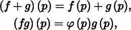
Let M be a regular surface. The set of smooth functions on M is denoted by C ^∞(M). We make C ^∞(M) into both a vector space over ℝ and a ring by defining operations as follows: for all functions f, g in C ^∞(M) and all real numbers c, let

and

for all p in M. The identity element of the ring is the constant function 1 _M that sends all points in M to the real number 1.

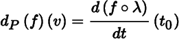
Let f be a function in C ^∞(M), and let p be a point in M. The differential of f at p is the map

defined by

(11.5.1)

for all vectors v in T _p (M), where λ(t) : (a, b) → M is any smooth curve such that λ(t ₀) = p and (dλ/dt)(t ₀) = v for some t ₀ in (a, b).

The next result is a counterpart of Theorem 10.1.3.

11.6 Maps on Regular Surfaces inℝ³

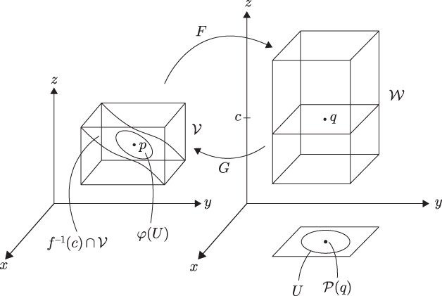
Let M and N be regular surfaces, let F : M → N be a smooth map, and let p be a point in M. The differential of F at p is the map

defined by

(11.6.1)

for all vectors v in T _p (M), where λ(t) : (a, b) → M is any smooth curve such that λ(t ₀) = p and (dλ/dt)(t ₀) = v for some t ₀ in (a, b). See Figure 11.6.1.

The next result is a generalization of Theorem 11.3.3.

11.7 Vector Fields Along Regular Surfaces in ℝ³

Let M be a regular surface, let V: M → ℝ³ be a map, and let p be a point in M. In the present context, we refer to V as a vector field along M . We say that V vanishes at p if V _p = (0, 0, 0), is nonvanishing at p if V _p  ≠ (0, 0, 0), and is nowhere‐vanishing (on M) if it is nonvanishing at every p in M.

Let us denote by the set of smooth vector fields along M. Then is nothing more than the set of (extended) smooth maps from M to ℝ³ . With operations on defined in a manner analogous to those in Section 10.3, is a vector space over ℝ and a module over C ^∞(M). We say that a vector field X: M → ℝ³ along M is a (tangent) vector field on M if X _p is in T _p (M) for all p in M. The set of smooth vector fields on M is denoted by Clearly, In fact, is a vector subspace and a C ^∞(M)‐submodule of . As an example, for a regular surface that has a covering chart, each of the components of the corresponding coordinate frame is a tangent vector field.

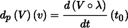
Let M be a regular surface, let V be a vector field in and let p be a point in M. The differential of V at p is the map

defined by

(11.7.1)

for all vectors V in T _p (M), where λ(t) : (a, b) → M is any smooth curve such that λ(t ₀) = p and (dλ/dt)(t ₀) = v for some t ₀ in (a, b). Observe that this is not a special case of (11.6.1) because ℝ³ is not a regular surface.