16.1 Exterior Derivatives

Let M be a smooth m‐manifold and recall that C ^∞(M) = Λ⁰(M) and . The exterior derivative of Section 15.4 can therefore be expressed as

According to Theorem 15.4.6, d is linear and satisfies a type of product rule. In this section, we describe a generalization of d that has corresponding properties. Three equivalent approaches to this theory are available—axiomatic, local, and global.

We observe that when s ≥ m,  Λ ^m (M) is the zero vector space, in which case d is the zero map. For any function f in C ^∞(M) = Λ⁰(M) and any form ω in Λ ^s (M), we have from (15.8.3) that fω = f ∧ ω , and then from Theorem 16.1.2 (b) that

(16.1.1)

Theorem 16.1.2 will be used often, usually without attribution.

The next result is a generalization of Theorem 15.11.2.

The following three examples show that the exterior derivative is related to the classical curl, gradient, and divergence operators presented in Section 10.6.

We close this section with two computations relevant to electrodynamics that will be needed in Section 22.2.

16.2 Tensor Derivations

A tensor derivation on a smooth manifold M is a family of linear maps

defined for r,  s ≥ 0 such that for all tensor fields in and ℬ in , and all (k,  l)‐contractions :

[D1]

[D2]

[D1] is a type of product rule for tensor fields, and [D2] says that “contraction commutes with tensor derivation”.

Observe that in the preceding computations, we implicitly used Theorem 15.7.2 to identify with a map in . The next result generalizes Example 16.2.3 using the same approach.

16.3 Form Derivations

A form derivation on a smooth manifold M is a family of linear maps

defined for s ≥ 0 such that

(16.3.1)

for all forms ω in Λ ^s (M) and ξ in .

16.4 Lie Derivative

Let M be a smooth manifold, let X be a vector field in , and consider the map defined by ℒ _X (Y) = [X,  Y] for all vector fields Y in . By parts (c) and (d) of Theorem 15.3.2, ℒ _X is linear and satisfies ℒ _X (fY) = X(f)Y + fℒ _X (Y) for all functions f in C ^∞(M) and all vector fields Y in . It follows from Theorem 16.2.7 that there is a unique tensor derivation

on M, called the Lie derivative with respect to X , such that

(16.4.1)

for all functions f in C ^∞(M) and all vector fields Y in , where has been abbreviated to ℒ _X .

The Lie derivative enjoys a wealth of algebraic properties.

We note that Jacobi's identity in part (e) of Theorem 15.3.2 gives rise to a product rule for Lie brackets in part (e) of the above theorem. The next result contains a product rule for tensor products, and the one after that a product rule for wedge products.

16.5 Interior Multiplication

The following definitions are the manifold versions of those appearing in Section 7.4. Let M be a smooth manifold, and let X be a vector field in . Interior multiplication by X is the family of linear maps

defined for s ≥ 2 by

for all forms ω in Λ ^s (M) and all vector fields Y ₁,   … ,  Y _s − 1 in . Recalling from (15.8.1) and (15.8.2) that and Λ⁰(M) = C ^∞(M), we extend the preceding definition to s = 1 as follows:

is given by

(16.5.1)

for all covector fields ω in . In particular, for any function f in C ^∞(M), we have from Theorem 15.4.5(b) and (16.5.1) that

(16.5.2)

For s = 0, we trivially define i _X  = 0; that is,

(16.5.3)

for all functions f in C ^∞(M).

We have defined two differential operators on smooth manifolds—the exterior derivative and the Lie derivative. Despite their evident differences in construction and properties, they are related by a remarkable identity that involves interior multiplication.

The next result is a generalization of Theorem 16.4.6.

16.6 orientation

The material in this section borrows heavily from Section 8.2 and Section 12.7. Let M be a smooth manifold, let (U,  (x ⁱ )) and be overlapping charts on M, and let and be the corresponding coordinate frames. Recall from Section 8.2 that for a given point p in , the coordinate bases and are said to be consistent if

We say that (U,  (x ⁱ )) and are consistent if and are consistent for all p in . A smooth atlas for M is said to be consistent if every pair of overlapping charts in is consistent.

A pointwise orientation of M is a collection of orientations

(16.6.1)

one for each tangent space of M. Without additional structure, the orientations might vary erratically from point to point. We say that is a (smooth) orientation of M if there is a consistent smooth atlas for M such that for each chart (U,  (x ⁱ )) in and corresponding coordinate frame ,

(16.6.2)

all p in U, where we recall that is the equivalence class of all bases for T _p (M) (not just coordinate bases) that are consistent with . Let (U,  (x ⁱ )) and be overlapping charts in , let and be the corresponding coordinate frames, and let p be a point in . Since the charts are consistent, , hence (16.6.2) is independent of the choice of chart in at p.

Suppose is in fact an orientation of M. The existence of a consistent smooth atlas for M ensures that the orientations in vary “smoothly” on M. We refer to the pair as an oriented smooth manifold. The notation , and sometimes , is used as an alternative to . Each chart in is said to be positively oriented (with respect to ).

According to terminology introduced in Section 8.2, for each point p in M, we say that each basis in is positively oriented [with respect to ].

Let M be a smooth manifold, and let be a consistent smooth atlas for M. Then (16.6.1) and (16.6.2) can be used to define a corresponding orientation of M, called the orientation induced by . The remarks above show that the orientation is well‐defined. We say that a smooth manifold is orientable if it has a consistent smooth atlas. Evidently, the concept of an orientation of a smooth manifold and that of a consistent smooth atlas for a smooth manifold are closely related, almost to the extent of being indistinguishable.

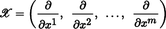
Let be an oriented smooth m‐manifold, let (U,  (x ¹,   … ,  x ^m )) be a chart in , and let

be the corresponding coordinate frame. Then

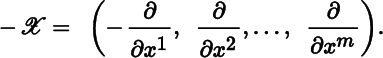
is a chart on M, and the corresponding coordinate frame is

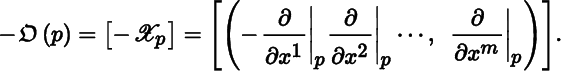
It is easily shown using Theorem 14.3.5(b) that

is a consistent smooth atlas for M. The orientation of M induced by is

where

We say that the orientation is the opposite of .

A vector space always has precisely two orientations, but the situation is different for smooth manifolds. As we saw in Example 12.7.9, the Möbius band does not have a smooth unit normal vector field, and therefore, by Theorem 12.7.6, it fails to have an orientation. On the other hand, if a smooth manifold has an orientation, then it has at least two of them, namely, the given orientation and its opposite—but there could be more.

Defining the orientation of a smooth manifold in terms of an atlas ultimately rests on the way the bases for tangent spaces are oriented, which is geometrically appealing. However, this approach is not computationally convenient. We now present an algebraic alternative that eases this problem, but at the expense of greater abstraction.

Let M be a smooth m‐manifold. We say that a form ϖ in Λ ^m (M) is an orientation form (on M) if it is nowhere‐vanishing; or equivalently, if ϖ _p is a nonzero multicovector in Λ ^m (T _p (M)) for all p in M; or equivalently, if ϖ _p is an orientation multicovector on T _p (M) for all p in M. In the literature, such a form is often referred to as a volume form, but we reserve this terminology for a particular type of orientation form that makes it possible (in certain settings) to measure “volume”. As we will soon see, there is no guarantee that a given smooth manifold has an orientation form.

Let M be a smooth manifold, and let ϖ and ϑ be orientation forms on M. By Theorem 16.6.1(a), there is a uniquely determined nowhere‐vanishing function f in C ^∞(M) such that ϖ = fϑ . We say that ϖ and ϑ are consistent (on M), and write ϖ ∼ ϑ , if f is strictly positive on M. It is easily shown that ∼ is an equivalence relation on the set of orientation forms on M. The equivalence class containing ϖ is denoted by [ϖ]. Since ϖ and −ϖ are not consistent, [ϖ] and [−ϖ] are distinct equivalence classes. We emphasize again that there is no guarantee that a given smooth manifold has even one orientation form, so the preceding equivalence relation may be vacuous. On the other hand, if the equivalence relation does exist, there could be more than two equivalence classes.

It was remarked in the introduction to this section that if a smooth manifold has an orientation, then it has at least two of them. The next result gives a condition under which there are two orientations, and no more.

It follows from Theorem 14.1.3 that a smooth manifold has countably many connected components, each of which is an open set in the smooth manifold. Let M be a smooth manifold that has a finite number of connected components C ₁,   … ,  C _k . Suppose C _i , viewed as an open submanifold of M, is orientable for i = 1,   … ,  k . Then C _i can be given an orientation independently of the other connected components. Taken together, the give an orientation of M, which we denote by . It follows from Theorem 16.6.8 that by taking all combinations of signs in we obtain the 2 ^k possible orientations of M.

Let be an oriented smooth ‐manifold, where , and let M be a submanifold of . In general, there is no mechanism for constructing an orientation of M from . However, when M is a hypersurface of , this may be possible, as the next result shows.

A couple of remarks on Theorem 16.6.9 are in order. First, although is independent of the choice of orientation form ϖ on that induces , the same cannot be said for the choice of nowhere‐tangent vector field V in . In particular, the orientation induced by . Second, without further assumptions, there is no guarantee that a nowhere‐tangent vector field in exists in the first place, an issue we return to in Theorem 19.11.1.

Let and be oriented smooth m‐manifolds, and let be a diffeomorphism. We say that F is orientation‐preserving if : is orientation‐preserving as a linear map for all p in M.

16.7 Integration of Differential Forms

In this section, we introduce the theory of integration on smooth manifolds. It may come as a surprise to learn that in this setting the objects to be integrated are not functions but rather differential forms. In order for integration of functions to be possible, we need a type of smooth manifold that has structure beyond what has been considered up to now. This topic is covered in Section 19.10.

Let M be a smooth m‐manifold, and let ω be a form in Λ ^m (M). The support of ω is denoted by supp(ω) and defined to be the closure in M of the set of points at which ω is nonvanishing:

We say that ω has compact support if supp(ω) is compact in M. Let U be an open set in M. It is said that ω has support in U if supp(ω) ⊆ U and that ω has compact support in U if supp(ω) ⊆ U and supp(ω) is compact in M.

We begin by defining the integral of differential forms in the setting of Euclidean spaces and then generalize to smooth manifolds.

Let V be an open set in ℝ ^m , and let ω be a form in Λ ^m (V) that has compact support. By Theorem 15.8.5, ω can be expressed as

(167.1.)

where f is a uniquely determined function in C ^∞(V). Since f is smooth, by Theorem 10.1.1, it is continuous, and from

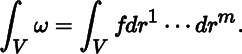
it follows that f has compact support. We have from (10.5.3) and the associated discussion that the integral of f over V exists and is denoted by ∫ _V fdr ¹⋯dr ^m . The integral of ω over V is denoted by ∫ _V ω and defined by

(16.7.2)

We can express the preceding identity more suggestively as

The next result shows that the integral is independent of the way the form is parametrized.

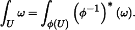
We now generalize to smooth manifolds. Let be an oriented smooth m‐manifold, and let ω be a form in Λ ^m (M) that has compact support. We first consider the case where ω has compact support in the coordinate domain of a single chart (U,  φ = (x ⁱ )) in . Viewing φ(U) as a smooth manifold, it can be shown that the form (φ ⁻¹)^*(ω) in Λ ^m (φ(U)) has compact support in the open set φ(U) in ℝ ^m _. In keeping with (16.7.2), the integral of ω over U is denoted by ∫ _U ω and defined by

(16.7.3)

It can be shown that ∫ _U ω does not depend on the choice of chart with coordinate domain containing supp(ω).

Let us look more closely at the right‐hand side of (16.7.3). By Theorem 15.8.5, ω can be expressed in local coordinates as

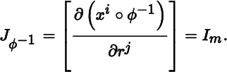
where f is a uniquely determined function in C ^∞(U). It follows from Theorem 14.8.5(a) that φ ⁻¹ : φ(U) → U is smooth. Since

hence r ⁱ  = x ⁱ  ∘ φ ⁻¹ , we have from (15.13.3) that the corresponding Jacobian matrix is

Then Theorem 15.13.3(b) gives

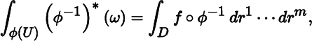
Using (10.5.3), (16.7.1), and (16.7.2), the right‐hand side of (16.7.3) can now be expressed as

where D is any compact domain of integration in ℝ ^m such that supp ((φ ⁻¹)^*(ω)) ⊆ D ⊂ φ(U).

Using a partition of unity argument, we now address the case where ω does not have compact support in the coordinate domain of a single chart in . It is clear that the union of the coordinate domains of all charts in comprises an open cover of supp(ω). Since ω has compact support, supp(ω) has a finite open cover consisting of the coordinate domains of a finite number of charts in . Let {π _i  : i = 1,   … ,  k} be a partition of unity subordinate to . 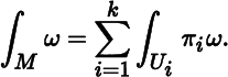It can be shown that the form π _i ω in Λ ^m (M) has compact support in U _i . Thus, definition (16.7.3) applies and each integral exists. The integral of ω over M is denoted by ∫ _M ω and defined by

It can be shown that ∫ _M ω does not depend on the choice of open cover or the choice of partition of unity.

Integration of differential forms has the properties desired of an integral.

16.8 Line Integrals

Due to its endpoints, a closed interval [a, b] in ℝ is not a smooth 1‐manifold. However, as discussed in Section 17.1, [a, b] is what we will later refer to as a smooth 1‐manifold with boundary. For present purposes, it is convenient to ignore the distinction and treat [a, b] as a smooth 1‐manifold.

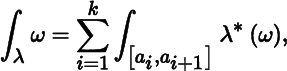
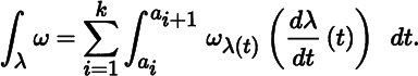
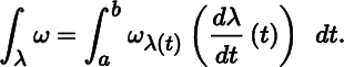
Let M be a smooth manifold, and let λ(t) : [a,  b] → M be a (not necessarily smooth) curve. We say that λ is piecewise smooth if there is a finite series of real numbers a = a ₁ < a ₂ < ⋯ < a _k + 1 = b such that the restriction of λ to [a _i ,  a _i + 1] is a smooth curve for i = 1,   … ,  k . Suppose λ is in fact piecewise smooth, and let ω be a covector field in . Motivated by (16.7.3), the line integral of ω over λ is denoted by ∫ _λ ω and defined by

(16.8.1)

where the ith integrand on the right‐hand side is interpreted as the restriction of λ ^*(ω) to [a _i ,  a _i + 1]. When λ is smooth, (16.8.1) simplifies to

(16.8.2)

Clearly, [a _i ,  a _i + 1] is a domain of integration in ℝ, and by Theorem 9.4.2, it is compact for i = 1,   … ,  k . It follows from Theorem 15.11.8, that

(16.8.3)

When λ is smooth, (16.8.3) simplifies to

(16.8.4)

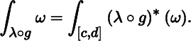
Let g(u) : [c,  d] → [a,  b] be a diffeomorphism, and let c _i  = g ⁻¹(a _i ) for i = 1,   … ,  k + 1. According to Theorem 10.2.4(c), g is either strictly increasing or strictly decreasing, so we have either c = c ₁ < c ₂ < ⋯ < c _k + 1 = d or c = c _k + 1 < c _k  < ⋯ < c ₁ = d . From (16.8.1), the line integral of ω over λ ∘ g is

(16.8.5)

where

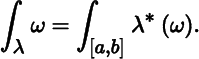
for i = 1,   … ,  k . When λ is smooth, (16.8.5) simplifies to

(16.8.6)

The next result is the line integral counterpart of Theorem 16.7.1.

Theorem 16.8.1 says that, up to a sign determined by the “direction” of the reparametrizing diffeomorphism, the line integral of ω is independent of the way λ is parametrized.

The next result can be viewed as a generalization of the fundamental theorem of calculus.

16.9 Closed and Exact Covector Fields

Let M be a smooth manifold, and let ω be a covector field in . We say that ω is closed if d(ω) = 0, exact if there is a function f in C ^∞(M) such that ω = d(f), conservative if ∫ _λ ω = 0 for all piecewise smooth curves λ(t) : [a,  b] → M such that λ(a) = λ(b), and path‐independent if ∫ _μ ω = ∫ _ψ ω for all piecewise smooth curves μ(t) : [a,  b] → M and ψ(u) : [c,  d] → M such that μ(a) = ψ(c) and μ(b) = ψ(d). In this section, we explore the various ways in which these properties are related.

In light of Theorem 16.9.3, there are three possibilities for a covector field with respect to being exact or not, and closed or not: (i) exact (hence closed), (ii) closed and not exact, and (iii) not closed (hence not exact). The following examples illustrate each of these cases.

Let M be a smooth manifold, and let ω be a form in Λ ^s (M). Generalizing earlier definitions, we say that ω is closed if d(ω) = 0, and exact if there is a form ξ in Λ ^s − 1(M) such that ω = d(ξ).

Theorem 16.9.3 has an immediate generalization.

Recall that a subset S of ℝ ^m is said to be star‐shaped about a point p ₀ in S if tp + (1 − t)p ₀ is in S for all p in S and all t in [0, 1]; that is, for all p in S , the line segment joining p ₀ to p is contained in S .

Theorem 16.9.8 explains why the form in Example 16.9.6 is not exact: the punctured plane is not star‐shaped about the origin.

16.10 Flows

We saw in Section 15.1 that the velocity of a smooth curve on a smooth manifold is a vector field on the curve. In this section, we turn this observation around and ask if a given smooth vector field on a smooth manifold can be realized as a family of velocities of smooth curves.

Let M be a smooth manifold, let X be a vector field in , and let p be a point in M . An integral curve of X with starting point p is a smooth curve λ(t) : (a,  b) → M such that

for all t in (a,  b). We say that λ is maximal if it cannot be extended to a smooth curve satisfying these properties on a larger open interval.

Continuing with the above setup, let Φ _p (t) : (a _p , b _p ) → M be the maximal integral curve of X with starting point p . The maximal flow domain is defined by

and the maximal flow of X is the map Φ : D → M defined by

for all (t,  p) in D . For each t in ℝ, let

and consider the map

defined by

for all p in M _t . We note that for sufficiently large t, M _t might be empty.

In physical terms, M _t is the set of points p in M for which a “particle” starting at p is able to “flow” for t units under the “action” of Φ. It is helpful to visualize Φ _t as a map that causes a portion of the vector field to “flow” bodily across the underlying smooth manifold for a “distance” of t units. We observe that with the above definitions,

(16.10.3)

Theorem 16.10.3 says that the maximal integral curves corresponding to a vector field combine to form a smooth map defined on an open set, and that the flow of particles referred to above takes place in a “diffeomorphic” fashion.

We close this section with a pair of results that demonstrate the surprisingly close connection between maximal flows and Lie derivatives.

The second right‐hand side of (16.10.4) allows us to think of ℒ _X (Y) _p as a type of “directional derivative” of Y in the “direction” X _p , in the following sense. Ordinarily there is no connection between vectors in T _p (M) and those in other tangent spaces of M . The maximal flow of X establishes a link between T _p (M) and those tangent spaces of M that correspond to points that lie on the maximal integral curve with starting point p . To find ℒ _X (Y) _p , the diffeomorphism Φ _t is used to compute the pullback of Y at p , yielding a vector (Φ _t )^*(Y) _p in T _p (M), which is then compared with Y _p by taking a limit. This makes sense because all computations are performed in T _p (M).

In Section 16.4, the Lie derivative was formulated as a tensor derivation. In particular, the Lie derivative of a vector field was defined in terms of the Lie bracket. It is more usual in the literature for the Lie derivative of a vector field to be defined using the first equality in (16.10.4). Theorem 16.10.5 shows that the two approaches are equivalent.