In this chapter, we review some of the basic results from the theory of matrices and determinants.
2.1 Matrices
Let us denote by Matm × n the set of m × n matrices (that is, m rows and n columns) with real entries. When m = n, we say that the matrices are square. It is easily shown that with the usual matrix addition and scalar multiplication, Matm × n is a vector space, and that with the usual matrix multiplication, Matm × m is a ring.
Let P be a matrix in Matm × n, with
The transpose of P is the matrix PT in Matn × m defined by
The row matrices of P are
and the column matrices of P are
We say that a matrix
in Matm × m is symmetric if Q = QT, and diagonal if
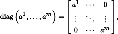
for all i ≠ j. Evidently, a diagonal matrix is symmetric. Given a vector (a1, … , am) in ℝm, the corresponding diagonal matrix is defined by
where all the entries not on the (upper‐left to lower‐right) diagonal are equal to 0. For example,
The zero matrix in Matm × n, denoted by Om × n, is the matrix that has all entries equal to 0. The identity matrix in Matm × m is defined by
so that, for example,
We say that a matrix Q in Matm × m is invertible if there is a matrix in Matm × m, denoted by Q–1 and called the inverse ofQ, such that
It is easily shown that if the inverse of a matrix exists, then it is unique.
Multi‐index notation, introduced in Appendix A, provides a convenient way to specify submatrices of matrices. Let 1 ≤r ≤ m and 1 ≤s ≤ n be integers, and let I = (i1, … , ir) and J = (j1, … , js) be multi‐indices in
and
respectively. For a matrix
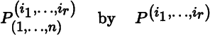
in Matm × n, we denote by
the r × s submatrix of P consisting of the overlap of rows i1, i2, … , ir and columns j1, j2, … , js (in that order); that is,
When r = m, in which case (i1, … , im) = (1, … , m), we denote
and when s = n, in which case (j1, … , jn) = (1, … , n), we denote
When r = 1, so that I = (i) for some 1 ≤ i ≤ m, we have
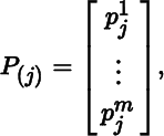
which is the ith row matrix of P. Similarly, when s = 1, so that J = (j) for some 1 ≤ j ≤ n, we have
which is the jth column matrix of P.
For a matrix
in Matm × m, the trace of P is defined by
2.2 Matrix Representations
Matrices have many desirable computational properties. For this reason, when computing in vector spaces, it is often convenient to reformulate arguments in terms of matrices. We employ this device often.
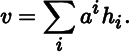
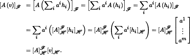
Let V be a vector space, let ℋ = (h1, … , hm) be a basis for V, and let v be a vector in V, with
The matrix representation of v with respect to ℋ is denoted by [v]ℋ and defined by
We refer to a1, … , am as the components of v with respect to ℋ. In particular,
(2.2.1)
where 1 is in the ith position and 0s are elsewhere for i = 1, … , m.
With V and ℋ as above, let W be another vector space, and let
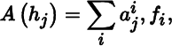
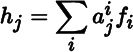
be a basis for W. Let A : V → W be a linear map, with
(2.2.2)
so that
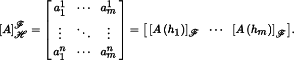
for j = 1, … , m. The matrix representation of A with respect to ℋ and ℱ is denoted by
and defined to be the n × m matrix
(2.2.3)
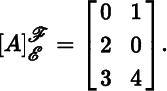
As an example, consider the linear map A : ℝ2 → ℝ3 given by A(x, y) = (y, 2x, 3x + 4), and let ℰ and ℱ be the standard bases for ℝ2 and ℝ3, respectively. Then
By parts (a) and (b) of Theorem 2.2.2,
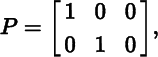
Let V be a vector space, and let ℋ and ℱ be bases for V. Setting A = idV in Theorem 2.2.4 yields
(2.2.5)
This shows that
is the matrix that transforms components with respect to ℋ into components with respect to ℱ. For this reason,
is called the change of basis matrix from ℋ to ℱ. Let
. Then (2.2.2) and (2.2.3) specialize to
(2.2.6)
for i = 1, … , m and
(2.2.7)
2.3 Rank of Matrices
Consider the n‐dimensional vector space Mat1 × n of row matrices and the m‐dimensional vector space Matm × n of column matrices. Let P be a matrix in Matm × n. The row rank of P is defined to be the dimension of the subspace of Mat1 × n spanned by the rows of P:
Similarly, the column rank of P is defined to be the dimension of the subspace of Matm × 1 spanned by the columns of P:
To illustrate, for
we have rowrank(P) = colrank(P) = 2. As shown below, it is not a coincidence that the row rank and column rank of P are equal.
In light of Theorem 2.3.2, the common value of the row rank and column rank of P is denoted by rank (P) and called the rank of P. Thus,
(2.3.1)
2.4 Determinant of Matrices
This section presents the basic results on the determinant of matrices.
Consider the m‐dimensional vector space Matm × 1 of column matrices and the corresponding product vector space (Matm × 1)m. We denote by (E1, … , Em) the standard basis for Matm × 1, where Ej has 1 in the jth row and 0s elsewhere for j = 1, … , m. Let
be an arbitrary function, and let σ be a permutation in Sm, the symmetric group on {1, 2, … , m}.We define a function
by
for all matrices P1, … , Pm in Matm × 1.
A function Δ : (Matm × 1)m → ℝ is said to be multilinear if for all matrices P1, … , Pm, Q in Matm × 1 and all real numbers c,
for i = 1, … , m. We say that Δ is alternating if for all matrices P1, … , Pm in Matm × 1,
for all 1 ≤ i < j ≤ m. Equivalently, Δ is alternating if τ(Δ) = − Δ for all transpositions τ in
.
A function Δ : (Matm × 1)m → ℝ is said to be a determinant function (on Matm × 1) if it is both multilinear and alternating.
Let P be a matrix in Matm × m, and recall that in multi‐index notation the column matrices of P are P(1), … , P(m). Setting
we henceforth view P as an m‐tuple of column matrices. In this way, the vector spaces Matm × m and (Matm × 1)m are identified. Accordingly, we now express the determinant function in Theorem 2.4.4 as
so that
where det (P) is referred to as the determinant of P. In particular, the condition det(E1, … Em) = 1 in Theorem 2.4.4 becomes
(2.4.2)
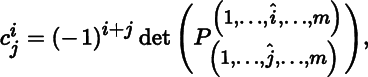
Let P be a matrix in Matm × m. The ij‐th cofactor of P is defined by
where ^ indicates that an expression is omitted. Thus,
is the matrix in Mat(m − 1) × (m − 1) obtained by deleting the ith row and jth column of P. The adjugate of P is the matrix in Matm × m defined by
The next result is not usually included in an overview of determinants, but it will prove invaluable later on.
It was remarked in connection with Theorem 2.2.3 that Matm × m is a ring under the usual operations of matrix addition and matrix multiplication, hence it is a group under matrix addition. But Matm × m is clearly not a group under matrix multiplication because not all matrices have an inverse. However, Matm × m contains a number of matrix groups. The largest of these is the general linear group, consisting of all invertible matrices:
where the characterization using determinants follows from Theorem 2.4.8.
We say that a matrix P in Matm × m is orthogonal if PTP = Im. If so, then PT = P−1, hence P PT = P P−1 = Im. Thus, PTP = Im if and only if P PT = Im.The orthogonal group is the subgroup of GL (m) consisting of all orthogonal matrices:
For a matrix P in O (m), we have
hence det(P) = ± 1. The special orthogonal group is the subgroup of O (m) consisting of all matrices with determinant equal to 1:
2.5 Trace and Determinant of Linear Maps
The trace and determinant of a matrix were defined in Section 2.1 and Section 2.4, respectively. We now extend these concepts to linear maps.
Let V be a vector space, let ℋ be a basis for V, and let A : V → V be a linear map. The trace of A is defined by


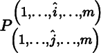 is the matrix in Mat(m − 1) × (m − 1)
obtained by deleting the ith row and jth column of P. The adjugate of P
is the matrix in Mat
m × m
defined by
is the matrix in Mat(m − 1) × (m − 1)
obtained by deleting the ith row and jth column of P. The adjugate of P
is the matrix in Mat
m × m
defined by