Orientation is concerned with “sidedness”, a concept that is intuitively obvious but surprisingly difficult to formulate in a mathematically rigorous fashion. In Section 8.1, we make a few observations based on concrete examples, and then present a preliminary definition of orientation for ℝ ^m . In Section 8.2, these ideas are developed into a computational framework for arbitrary vector spaces using our recently acquired knowledge of multicovectors.

8.1 Orientation of ℝ ^m

Let be a basis for ℝ ^m . Corresponding to each point in ℝ ^m is an m‐tuple of real numbers consisting of the components of the point with respect to . For m = 1, 2, 3, we can plot this m‐tuple on a rectangular coordinate system, with axes labeled h ₁,…,h _m . We use the geometry of this approach to motivate a definition of orientation.

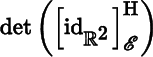
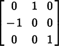
Consider the bases ℰ = (e ₁, e ₂), (e ₂, − e ₁), and (e ₂, e ₁) for ℝ² , where ε is the standard basis. In Figures 8.1.1(a)–(c), these bases are depicted as the axes of rectangular coordinate systems. The configuration in Figure 8.1.1(a), which we call the standard configuration for ℝ² , is said to have a counterclockwise orientation because the 90° rotation taking e ₁ to e ₂ is in a counterclockwise direction. The configuration in Figure 8.1.1(b) is also said to have a counterclockwise orientation because its axes can be rigidly rotated about the origin to give the same configuration as in Figure 8.1.1(a). On the other hand, the configuration in Figure 8.1.1(c) is said to have a clockwise orientation because its axes cannot be rigidly rotated in such a fashion (or equivalently, because the 90° rotation taking e ₁ to e ₂ is in a clockwise direction). These observations are summarized in the first three columns of Table 8.1.1.

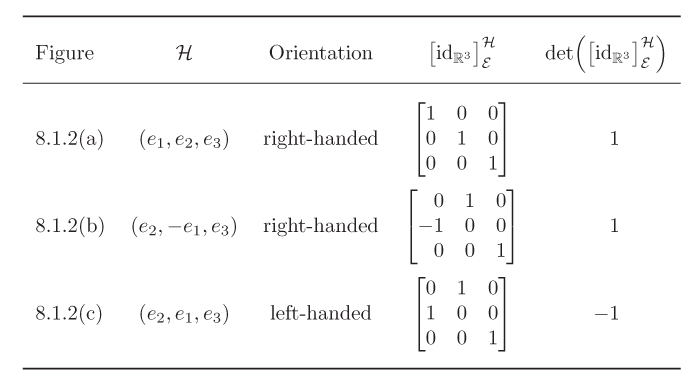
Now consider the bases ℰ = (e ₁, e ₂, e ₃), (e ₂, − e ₁, e ₃), and (e ₂, e ₁, e ₃) for ℝ³ , where ℰ is the standard basis. In Figures 8.1.2(a)–(c), these bases are depicted

as the axes of rectangular coordinate systems. The configuration in Figure 8.1.2(a), which we call the standard configuration for ℝ³ , is said to have a right‐handed orientation because you can grasp the positive e ₃‐axis in your right hand, with your thumb pointing along the positive e ₃‐axis and your fingers curled around the e₃‐axis in a counterclockwise direction with respect to the e ₁ e ₂‐plane. The configuration in Figure 8.1.2(b) is also said to have a right‐handed orientation because its axes can be rigidly rotated to give the same configuration as in Figure 8.1.2(a). On the other hand, the configuration in Figure 8.1.2(c) is said to have a left‐handed orientation because it cannot be rigidly rotated in such a fashion (or equivalently, because you can grasp the positive e ₃‐axis in your left hand, with your thumb pointing along the positive e ₃‐axis and your fingers curled around the e ₃‐axis in a clockwise direction with respect to the e ₁ e ₂‐plane). These observations are summarized in the first three columns of Table 8.1.2.

In the tables, we also give the change of basis matrix that takes the standard basis ℰ to the basis , as well as the value of its determinant. The crucial observation is that for these examples, orientation is preserved when (and only

when) the change of basis matrix has a positive determinant. This provides a rationale for the following general definition of orientation in ℝ ^m .

Let ℰ and be bases for ℝ ^m , where E is the standard basis. It follows from Theorem 2.4.12 that . We say that has the standard orientation if

(8.1.1)

In particular, ℰ has the standard orientation.

8.2 Orientation of Vector Spaces

In Section 8.1, we defined what it means for a basis for ℝ ^m to have a certain orientation by comparing it with the standard basis. This approach to orientation works in ℝ ^m because there is an obvious choice of reference basis, something that may not be the case for an arbitrary vector space.

Let V be a vector space of dimension m, and let and ℱ be bases for V. It follows from Theorem 2.4.12 that . We say that and ℱ are consistent, and write ˜ ℱ, if

Using Theorem 2.2.2(c) and Theorem 2.2.5(b), it is easily shown that ˜ is an equivalence relation on the set of bases for V, and that there are precisely two equivalence classes. Each equivalence class is said to be an orientation of V . The equivalence class containing a given basis is denoted by []. Let ℋ = (h ₁, h ₂, …, h _m ), and let

(8.21)

Clearly, – is a basis for V and , so and – are not consistent. We say that the orientation [–] is the opposite of []. Thus, for any basis for V, the orientations of V are [] and [–]. For example, the orientations of ℝ ^m are [ℰ] and [–ℰ], where ℰ is the standard basis for ℝ ^m . We refer to [ℰ] as the standard orientation of ℝ ^m . According to this terminology, ℰ is a basis in the standard orientation, which is somewhat different from Section 8.1 where ℰ was said to have the standard orientation. It is convenient to adopt this language more generally: for any vector space, a basis in an orientation is said to have that orientation.

Once an orientation of V has been chosen, the pair (V, ) is called an oriented vector space, and V is said to have the orientation . The alternative orientation is denoted by – and called the opposite of . If a basis for V is in , it is said to be positively oriented (with respect to ). We will often find it convenient to say, for instance, that “ is a basis for V that is positively oriented with respect to ” rather than the more concise “ is in ”. Although convention or circumstances tend to influence the orientation assigned to a given vector space, it needs to be emphasized that ultimately the decision is a matter of choice. There is nothing intrinsic to or – that makes one preferable to the other as an orientation of V. Having said that, in the case of ℝ ^m we adopt the following convention.

Throughout, ℝ ^m is assumed to have the standard orientation.

We now present an equivalent approach to orientation using multicovectors. Let V be a vector space of dimension m. In the present context, a nonzero multicovector in Λ ^m (V) is called an orientation multicovector on V. As an example, let (h ₁,…,h _m ) be a basis for V, and let (h ₁,…, h _m ) be its dual basis. By Theorem 7.2.9, θ ¹ ∧ … ∧ θ ^m (h ₁, …, h _m ) = 1 , so θ ¹ ∧ … ∧ θ ^m is an orientation multicovector on V. More generally, we have the following result.

Let V be a vector space, and let ϖ and ϑ be orientation multicovectors on V. By Theorem 7.2.12(d) and Theorem 8.2.1, ϖ spans Λ ^m (M) (as does ϑ). It follows that ϖ = cϑ for some nonzero real number c. We say that ϖ and ϑ are consistent, and write ϖ˜ϑ , if c > 0. It is easily shown that ˜ is an equivalence relation on the set of orientation multicovectors on V, and that there are precisely two equivalence classes. The equivalence class containing ϖ is denoted by [ϖ]. By definition, [ϖ] comprises all multicovectors on V that are consistent with ϖ . Evidently, ϖ and −ϖ are not consistent. Thus, for any orientation multicovector ϖ on V, the equivalence classes of orientation multicovectors are [ϖ] and [−ϖ].

Let be a basis for V. It is clear that orientation multicovectors in the same equivalence class induce the same orientation, and that orientation multicovectors in different equivalence classes induce opposite orientations. We therefore have a bijective map

defined by assigning [ϖ] and [−ϖ] to the orientations induced by ϖ and −ϖ , respectively. This shows that we are free to specify orientations using either (equivalence classes of) bases for V or (equivalence classes of) orientation multicovectors on V. For purposes of computation, the latter approach is generally more convenient.

A remark is that, in contrast to part (c) of Theorem 8.2.5, the orientation induced on U is not independent of the choice of vector in . In particular, if v induces _U , then –v induces – _U .

8.3 Orientation of Scalar Product Spaces

In Section 8.2, we considered orientation of vector spaces. We now expand our coverage to include scalar product spaces.

Let (V, g, ) be an oriented scalar product space of dimension m ≥ 2, and let Ω _V be its volume multicovector. By Theorem 8.3.4, Ω _V induces . Let U be a subspace of V of dimension m – 1 on which g is nondegenerate. We have from Theorem 4.1.2(b) that U ^⊥ is a 1‐dimensional subspace of V, and from Theorem 4.1.3 that V = U ⊕ U ^⊥ .Let u be a unit vector in U ^⊥, so that ℝu = U ^⊥ , hence V = U ⊕ ℝu . Since g is nondegenerate on U, g| _U is a scalar product on U. By parts (a) and (b) of Theorem 8.2.5, i _u (Ω _V )| _U is an orientation multicovector on U that induces a certain orientation of U denoted by _U . Thus, is an oriented scalar product space of dimension m – 1. Let Ω _U be its volume multicovector. The question arises as whether the orientation multicovectors i _u Ω _U | _U and Ω _U are related. As the next result shows, they are one and the same.

8.4 Vector Products

In this section, we generalize the well‐known vector product in ℝ³ to an arbitrary scalar product space.

Let (V, g) be a scalar product space with signature (“₁, …, ” _m ), let ℰ = (e ₁, …, e _m ) be an orthonormal basis for V, and let v ₁, …, v _m − 1 be vectors in V. The vector product (or cross product) of v ₁, …, v _m − 1 (in that order) with respect to ℰ is defined by

(8.4.1)

where (i)^c is the multi‐index

Clearly, the vector product of given vectors depends on the order in which they are taken and the choice of orthonormal basis.

In this chapter, the vector product × on V is computed with respect to a given orthonormal basis ℰ for V.

Throughout, the vector product × on is computed with respect to the standard basis for .

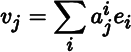
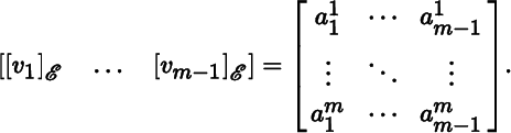
We obtain a computationally convenient alternative to (8.4.1) as follows. Let

for j = 1, …, m − 1, so that from (2.2.3),

(8.4.2)

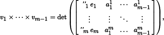
Then (8.4.1) can be expressed as the formal identity

(8.4.3)

provided we expand the “determinant” along the first column.

When m = 2, even though the notation for the left‐hand sides of (8.4.1) and (8.4.3) simplifies to a single vector, the right‐hand sides can still be computed. Let v = a ¹ e ₁ + a ² e ₂ . Then the “vector product” of v is

When the context is meaningful, this quantity has the same properties as a vector product when m ≥ 3.

The vector product has a number of interesting algebraic properties, several of which, not surprisingly, are expressed in terms of determinants and wedge products.

In light of Theorem 8.4.3(b), we drop parentheses and denote

The next result is the main reason for considering vector products.

At first glance, Theorem 8.4.4 appears to promise more than it actually delivers. To make the result truly informative, we need v ₁ × ⋯ × v _m − 1 to be a nonzero vector and U ^⊥ to be a 1‐dimensional subspace of V. These conditions can be met with further assumptions: see Theorem 8.4.8 and Theorem 8.4.10(a).

It was remarked above that the vector product depends on the order in which vectors are taken and the choice of orthonormal basis. According to Theorem 8.4.3(d), changing the order of vectors at most affects the sign of the resulting vector product. In view of (8.4.1), it might be expected that computing with respect to a different orthonormal basis would have a significant impact on results. As Theorem 8.4.4 shows, this is not necessarily the case: regardless of the choice of orthonormal basis, the vector product is always in the perp of the subspace spanned by the constituent vectors. In fact, several of the results to follow exhibit this same feature: see Theorem 8.4.5, Theorem 8.4.6, Theorem 8.4.8, and Theorem 8.4.9.

Theorems 8.4.3–8.4.7 are of little interest when the vector product equals the zero vector. The next result gives a straightforward condition that avoids this situation.

Whether vectors in a vector space are linearly independent or linearly dependent is unrelated to the presence or absence of a scalar product. This means that in Theorem 8.4.8, linear independence can be checked using any convenient choice of scalar product and orthonormal basis.

8.5 Hodge Star

In this section, we define a map that assigns to a given multicovector another multicovector that “complements” the first. The methods that result add to our growing armamentarium of techniques for computing with multicovectors.

Hodge star is the family of linear maps

defined for s ≤ m by the assignment

for all multicovectors n in Λ ^s (V). Let us denote

Theorem 8.5.2 provides a way to compute with ★ on an orthonormal basis for Λ ^S (V). Computations are then extended to all of Λ ^S (V) by the linearity of ★.