22.1 Linear Isometries on Lorentz Vector Spaces

Let (V, g, D) be an oriented Lorentz vector space, and let ε = (e ₁, …, e _m ) be an orthonormal basis for V that is positively oriented with respect to D. We denote by L _m the set of linear isometries on V:

where we recall that Lin(V, V) is the vector space of linear maps from V to V.

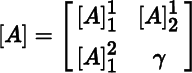
Let A be a map in Lin(V, V). For brevity, we denote by , and likewise omit &ip.eop; from the notation for other matrices. Corresponding to (4.4.1) and (4.4.2), we have

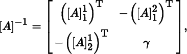
and

respectively, where

and

The ring isomorphism given by Theorem 2.2.3(b) restricts to a (multiplicative) group isomorphism between L and a subgroup of the general linear group GL(m) ⊂ Mult. In what follows, but without further mention, this group isomorphism is used to prove assertions about the group structure of L. In particular, we rely on the following: a subset of L is a subgroup if and only if the corresponding subset of GL(m) is a subgroup.

It follows from Theorem 22.1.2(d) that

(22.1.1)

Let us define

(22.1.2)

where we note that, by definition, γ and β have the same sign. Then

(22.1.3)

When which is the case of greatest interest,

Given a map A in Lm, we have from Theorem 4.4.3 that det(A) = ± 1, and from (22.1.1) that γ ≥ 1 or γ ≤ –1. Consider the sets

and

In the present context, an orientation‐preserving (orientation‐reversing) map is said to be proper (improper).

Let us recall the convention adopted in Section 4.9 that for a given orthonormal basis (e ₁, …, e _m ) for V, the future time cone T ⁺ is defined to be the one containing the timelike unit vector e _m .

In view of the preceding two results, we can characterize and as follows:

and

In the physics literature, is called the proper orthochronous Lorentz group on V.

Recall from Section 2.4 that the orthogonal group O(m) consists of all matrices P in Mat _m×m such that P ^T P = I _m , and the special orthogonal group SO(m) is the subgroup of O(m) consisting of those matrices P such that det(P) = 1.

We say that a map A in Lin(V, V) is a rotation (with respect to &ip.eop;) if is of the form

where is in SO(m – 1). By definition, det so det The set of rotations is

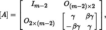
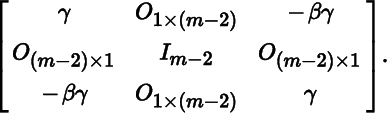
We say that a map A in Lin(V, V) is a boost (with respect to &ip.eop; in the (m – 1)st spacelike direction) if [A] is of the form

where and β is computed using (22.1.2). For convenience of notation, we have defined boosts in the (m – 1)st spacelike direction, but any other spacelike direction would do. For instance, a boost in the first spacelike direction takes the form

The set of boosts is

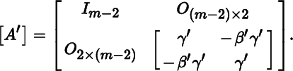
It is clear that Bm contains the identity map. Let A′ be another boost, with

Then

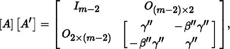
where

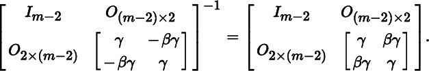
It is easily shown that and that and satisfy (22.1.2). Thus, is a boost. This demonstrates that Bm is closed under multiplication. However,

Since the matrix on the right‐hand side is missing the necessary minus signs to make it a boost, Bm does not contain inverses (except in the case of the identity map). Thus, Bm is not a group.

Based on Theorem 22.1.5, Theorem 22.1.6, Theorem 22.1.8, and Theorem 22.1.9, Figure 22.1.1 depicts the relationships between R _m , B _m , and as subsets of L _m , where the dot represents id _V .

Recall from Section 2.4 the vector space Mat _m × 1 of column matrices and its basis We make Mat _m × 1 into an oriented inner product space by choosing the orientation and defining the inner product using matrix multiplication as follows: for matrices P, Q in Mat _m × 1, the inner product is P ^T Q. Endowed with this structure, we identify Mat _m × 1 in an obvious way with the inner product space Rm.

We close this section by showing that any map in a proper orthochronous Lorentz group can be expressed as the composition of a rotation, followed by a boost, followed by another rotation.

22.2 Maxwell's Equations

Let (x, y, z, t) be standard coordinates on . In what follows, we think of x, y, z as “space” variables and t as a “time” variable. Using the differential operators in Section 10.6, an electromagnetic field in is characterized by Maxwell's equations:

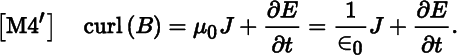
where the vector fields E, B, J in d are the electrical field, magnetic field, and current density, respectively; the function ρ in C ^∞ is the charge density; and the real numbers ɛ0 and μ0 are the permittivity of free space and the permeability of free space, respectively. We interpret the operators div and curl in the above identities as applying only to the space variables, and likewise for other vector calculus operators to follow. Let us assume units have been chosen so that , where is the speed of light. Thus, [M4] becomes

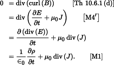
We observe that J and ρ are not independent of each other:

Then μ ₀∈₀ = 1 gives

(22.2.1)

which is called the continuity equation.

The rest of this section is devoted to finding alternative expressions for Maxwell's equations, especially in terms of differential forms. This is an opportunity to showcase some of the computational tools developed earlier.

Let us reformulate Maxwell's equations using what are referred to as potentials. It follows from Theorem 10.6.3 and [M2] that there is a vector field A in , called the magnetic potential, such that

(22.2.2)

Then [M3] gives

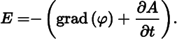
hence By Theorem 10.6.2, there is a function ϕ in called the electric potential, such that

so

(22.2.3)

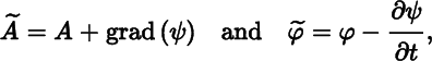
Equations (22.2.2) and (22.2.3) express E and B in terms of A and ϕ. As it stands, this representation is not unique. For example, let ψ be an arbitrary function in and let

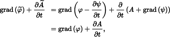
which is referred to as a gauge transformation of A and ϕ. Then

and by Theorem 10.6.1(c),

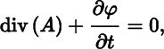
Thus, and also satisfy (22.2.2) and (22.2.3). The range of potentials is limited by the constraint

(22.2.4)

called the Lorenz gauge.

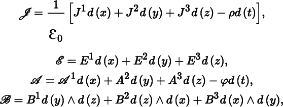
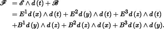
We now switch our focus from to and recast the preceding discussion in terms of differential forms. Let J = (J ¹, J ², J ³), E = (E ¹, E ², E ³), A = (A ¹, A ², A ³), and B = (B ¹, B ², B ³) , and define corresponding covector fields, , in * , and forms, in Λ² by

(22.2.6)

and

22.3 Einstein Tensor

Let (M, g) be a semi‐Riemannian manifold, and let ℛ be the Riemann curvature tensor. The Ricci curvature tensor (field) in is defined by

(22.3.1)

the scalar curvature (function) in C ^∞(M) is defined by

(22.3.2)

and the Einstein tensor (field) in defined by

In physics, the terms “Ricci curvature tensor”, “scalar curvature”, and “Einstein tensor” are typically used only when M is a Lorentz 4‐manifold, but we will continue with the more general context.

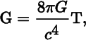
Adopting widely‐accepted units, Einstein's field equations for a Lorentz 4‐manifold are given by the tensor identity

where G is Newton's gravitational constant, c is the speed of light, and T is the so‐called stress–energy tensor. These 10 partial differential equations, which form the foundation of the general theory of relativity, describe the way gravity results from spacetime being curved by mass and energy. It is remarkable that the “left‐hand sides” of Einstein's equations are expressed entirely in geometric terms, in the sense that the Einstein tensor is completely determined by the metric of a Lorentz 4‐manifold.