In the introduction to Part III, we set out the task of developing a theory of differential geometry built upon our earlier study of curves and surfaces, but without having to involve an ambient space. Implicit in this undertaking was the aim of recovering, to the extent possible, the results presented for curves and surfaces. Chapters 14–17 have met significant parts of this agenda. Noticeably absent, however, is a discussion of “covariant derivative” and “metric”. We remedy the first of these deficits in this chapter by adding “connection” to our discussion of smooth manifolds.

18.1 Covariant Derivatives

Let M be a smooth manifold. A connection on M is a map

such that for all vector fields X, Y, Z in and all functions f in C ^∞(M) : [∇1] ∇ (X + Y, Z) =  ∇ (X, Z) +  ∇ (Y, Z).

We refer to the pair (M, ∇) as a smooth manifold with a connection. It is possible for a given smooth manifold to have more than one connection. Thus, a connection is not a fundamental constituent of the manifold in the same way that, for example, the boundary forms part of a smooth manifold with boundary.

In each of the preceding examples, we started with a “derivative” and used it to define a connection. Given a smooth manifold with a connection, we can reverse that process.

Let (M, ∇) be a smooth manifold with a connection, and let X be a vector Field in . We define a map

by

for all vector fields Y in . It follows from [∇3] and [∇4] that ∇ _X is ℝ ^m ‐linear, and from [∇4] that

for all functions f in C ^∞(M) and all vector fields Y in . By Theorem 16.2.7, there corresponds a unique tensor derivation

on M, called the covariant derivative with respect to X, where has been abbreviated to ∇ _X . In particular, we have

(18.1.1)

for all functions f in C ^∞(M).

Let (M, ∇) be a smooth manifold with a connection, and let X be a vector field in . It can be shown that ∇ _X is determined pointwise in the following sense: for all points p in M and all vector fields Y in ,

for all vector fields in such that . For each point p in M and vector v in T _p (M), we define a vector ∇ _v (Y) in T _p (M) by

(18.1.4)

where X is any vector field in such that X _p  = v . By Theorem 15.1.2, such an X always exists. Since ∇ _X is determined pointwise, ∇ _v (Y) is independent of the choice of vector field and is therefore well‐defined. It follows from (18.1.4) that for all vector fields X, Y in ,

(18.1.5)

for all p in M .

By definition, is the vector space of ℝ‐linear maps from the vector space to itself. We make into a ring over ℝ by defining multiplication to be composition of maps. Let Θ, ϒ, Ψ be three such maps, and define the bracket of Θ and ϒ by

It is easily shown that with this definition, is a Lie algebra over ℝ. In particular, Jacobi's identity is satisfied:

For vector fields X, Y, Z in , we have from parts (c) and (d) of Theorem 18.1.2 that ∇ _X , ∇ _Y , ∇ _Z are maps in , hence

(18.1.6)

18.2 Christoffel Symbols

In our study of regular surfaces in , we defined Christoffel symbols and used them to construct the covariant derivative, which we now think of as equivalent to a connection (see Example 18.1.1). Our approach to smooth manifolds with a connection proceeds in reverse: we start with a connection and then use it to define Christoffel symbols.

Let (M, ∇) be a smooth m‐manifold with a connection, let X be a vector field in , let (U, (x ⁱ )) be a chart on M , and let be the corresponding coordinate frame. It can be shown that ∇ restricts unambiguously to the smooth m‐manifold U . For simplicity of notation, let us denote the restriction

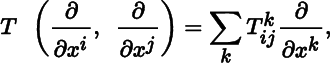
Then (U, ∇) is a smooth m‐manifold with a connection, (U, (x ⁱ )) is a covering chart on U , and is the corresponding coordinate frame. We can therefore express as

(18.2.1)

for i, j = 1, …, m , where the are uniquely determined functions in C ^∞(U), called the Christoffel symbols.

We observe that the expressions for ∇ _X (Y) and ∇ _X (ω) in parts (a) and (b) of Theorem 18.2.1 involve the α ⁱ but not their partial derivatives. In order to compute ∇ _X (Y) and ∇ _X (ω) at a given point, all we need to know about X is its value at that point. This is consistent with ∇ _X being determined pointwise, as was remarked in conjunction with (18.1.4).

In the notation of Theorem 18.2.1, we have as special cases

These formulas tell us that to take the covariant derivatives of Y and ω with respect to ∂/∂x ⁱ , we simply add a subscript “; i ” to each of the components in the local coordinate expressions.

We see from Theorem 15.6.3 and Theorem 18.2.3 that, despite appearances, the Christoffel symbols are not the components of a tensor. In classical terminology it is said that the Christoffel symbols “do not transform” like the components of a tensor.

18.3 Covariant Derivative on Curves

The definition of covariant derivative given in Section 18.1 refers to an entire smooth manifold. We now discuss a version of covariant derivative that applies only to smooth curves on a smooth manifold.

The above discussion is devoted to covariant derivatives on smooth curves. We close this section with an application to parametrized surfaces.

Let M be a smooth manifold, let σ(r, s) : (a, b) × (−ε, ε) → M be a parametrized surface, and let V be a vector field in . For a given point s in (−ε, ε), we define a vector field V _s in by V _s (r) = V(r, s), where we recall from Section 14.9 that the longitude curve σ _s (r) : (a, b) → M is defined by σ _s (r) = σ(r, s). The partial covariant derivative on σ with respect to r is the map

defined by

(18.3.2)

for all vector fields V in . The partial covariant derivative on σ with respect to s is defined similarly. As an example, we have from Theorem 15.1.5 that the vectors fields ∂σ/∂r and ∂σ/∂s are in . The partial covariant derivatives on σ with respect to r are

(18.3.3)

and the partial covariant derivatives on σ with respect to s are defined in a corresponding manner.

18.4 Total Covariant Derivatives

Let (M, ∇) be a smooth manifold with a connection. Total covariant derivative (or total covariant differential) is the family of linear maps

defined for r, s ≥ 0 by

(18.4.1)

for all tensor fields in , all covector fields ω ¹, …, ω ^r in , and all vector fields X, Y ₁, …, Y _s in . An alternative definition in the literature (not adopted here) is to place X last in the sequence of vector fields rather than first:

We say that is parallel (with respect to ∇) if . Let us denote

Let (U, (x ⁱ )) be a chart on M , and, in local coordinates, let have the components . The components of are denoted by

(not by , as might be expected from (18.4.1) and previous notation conventions).

We observe that the notation introduced in (18.2.2) and (18.2.3) is consistent with (18.4.2).

Adopting the notation of Theorem 18.4.7 and using (18.1.1) three times, we obtain

(18.4.3)

This shows that in the context of regular surfaces in is precisely , the second order covariant derivative of f with respect to X and Y , as given by (12.4.3).

18.5 Parallel Ranslation

Let (M, ∇) be a smooth manifold with a connection, and let λ : (a, b) → M be a smooth curve. We say that a vector field J in is parallel (with respect to ∇) if

for all t in (a, b).

At the beginning of this section, covariant differentiation along a curve was used to define parallel translation. The next result shows that parallel translation can be used to define covariant differentiation along a curve. In this sense, covariant differentiation and parallel translation are equivalent concepts.

18.6 Torsion Tensors

Let (M, ∇) be a smooth manifold with a connection. The torsion tensor (field) corresponding to ∇ is the map

defined by

(18.6.1)

for all vector fields X, Y in . We say that ∇ is symmetric (or torsion‐free) if T = 0; that is,

for all vector fields X, Y in .

Since T takes values in , referring to T as a “tensor field”, although usual in the literature, is not consistent with Theorem 15.7.2. We take up this matter in Section 19.5.

Let (M, ∇) be a smooth m‐manifold with a connection, and let (U, (x ⁱ )) be a chart on M . In local coordinates, T(∂/∂x ⁱ , ∂/∂x ^j ) can be expressed as

where the are uniquely determined functions in C ^∞(U).

18.7 Curvature Tensors

In this section, we generalize to smooth manifolds with a connection the Riemann curvature tensor on regular surfaces in .

Let (M, ∇) be a smooth manifold with a connection. The curvature tensor (field) is the map

defined by

(18.7.1)

for all vector fields X, Y, Z in . Since R takes values in , referring to R as a “tensor field”, although ubiquitous in the literature, presents the same issues of terminology encountered with the torsion tensor in Section 18.6. This concern will be addressed in Section 19.5.

Let (M, ∇) be a smooth m‐manifold with a connection, and let (U, (x ⁱ )) be a chart on M . In local coordinates, R(∂/∂x ⁱ , ∂/∂x ^j )∂/∂x ^k can be expressed as

(18.7.2)

where the are uniquely determined functions in C ^∞(U).

In the literature, the indexing of is sometimes defined by

This changes the indexing of certain identities, but has no substantive implications.

Let M be a smooth manifold (with or without a connection), let be a map, and define

for all vector fields X, Y, Z in . Thus, ∑_{(X, Y, Z)}ℱ(X, Y, Z) is a sum of terms obtained by permuting X, Y, Z cyclically. Clearly,

(18.7.3)

For example, Jacobi's identity for vector fields in , given by Theorem 15.3.2(e), can be expressed as

(18.7.4)

and Jacobi's identity for covariant derivatives in , defined by (18.1.6), becomes

(18.7.5)

For a map , where k > 3, we use the above notation, but apply the cyclic permutation only to the three arguments specified by the 3‐tuple under the summation sign, leaving the other arguments in place.

18.8 Geodesics

In this section, we introduce a type of “straight line” for smooth manifolds with a connection. A cardinal feature of straight lines in Euclidean space is that they give the shortest distance between distinct points. This is meaningless in the present setting because there is no notion of distance on a smooth manifold with a connection. However, in Newtonian physics, a particle with zero acceleration traces a straight line in Euclidean space. We make this observation our point of departure.

Let (M, ∇) be a smooth manifold with a connection, and let λ(t) : (a, b) → M be a smooth curve. Recall from Theorem 15.1.3 that the velocity of λ is the vector field dλ/dt in , and that λ is said to be regular if its velocity is nowhere‐vanishing. The acceleration of λ is defined to be the covariant derivative of the velocity, that is, the vector field (∇/dt)(dλ/dt) in . We say that λ is a geodesic if it has zero acceleration; that is,

for all t in (a, b); or equivalently, if dλ/dt is a parallel vector field in .

As an example, consider the straight line in ℝ³ parametrized by λ(t) = (t, t, t) : ℝ → ℝ³ The velocity and accelerations are (dλ/dt)(t) = (1,1,1) and (∇/dt)(dλ/dt)(t) = (0,0,0) for all t in ℝ³ , hence λ is a geodesic. Now consider the alternative parametrization : ℝ → ℝ³ Then and , so is not a geodesic. This illustrates that deciding whether a smooth curve is a geodesic depends not only on its “geometry” but also on its parametrization.

18.9 Radial Geodesics and Exponential Maps

Let (M, ∇) be a smooth manifold with a connection, let p be a point in M, and suppose T _p (M) has the standard smooth structure. Let ℰ _p be the set of vectors v in T _p (M) such that γ _{p, v} (1) is defined; that is, 1 is in the domain of γ _{p, v} , where γ _{p, v} is the maximal geodesic with starting point p and initial velocity v .

Continuing with the above setup, let v be a vector in ℰ _p . Using Theorem 18.9.2(c), we restrict γ _{p, v} to [0, 1] and obtain the geodesic

(18.9.1)

called the radial geodesic with starting point p and initial velocity v .

It follows from Theorem 18.8.2(a) that ρ _{p, v} (0) = p . By varying v , we obtain a family of radial geodesics with starting point p .

For the remainder of this section, we work toward a condition that ensures a uniqueness condition for radial geodesics.

Let (M, ∇) be a smooth m‐manifold with a connection, and let p be a point in M . The exponential map at p is the smooth map

defined by

(18.9.2)

for all vectors v in ℰ _p .

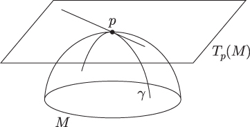
Roughly speaking, Theorem 18.9.3 says that the exponential function sends lines (or portions of lines) passing through the zero vector of the tangent space at a point to geodesics in the smooth manifold that pass through the point. See Figure 18.9.1.

By Theorem 14.8.4 and Theorem 18.9.1(a), ℰ _p is an open m‐submanifold of T _p (M), and from Theorem 14.3.3(b), we have the identification T _v (ℰ _p ) = T _v (T _p (M)) for each vector v in ℰ _p . The differential map of exp _p : ℰ _p  → M at v can therefore be expressed as

(18.9.4)

See Figure 18.9.2, and, for context, also see Figure 11.6.1. Let w be a vector in T _p (M), and consider the smooth curve μ _v (t) : (−ε, ε) → T _p (M) defined by μ _v (t) = v + tw . According to (14.7.4), (dμ _v /dt)(t) is a vector in . In the literature, (dμ _v /dt)(0) is sometimes denoted by w _v . Thus, w _v is a vector in T _v (T _p (M)), and it follows from (18.9.4) that d _v (exp _p )(w _v ) is a vector in . In geometric terms, we can think of T _v (T _p (M)) as the translation of T _p (M) to v , with w _v the corresponding translation of w . It is sometimes convenient to denote w _v simply by w and allow the underlying translation to be understood. As a further simplification, when v = 0, we use (14.3.4) to identify T ₀(T _p (M)) with T _p (M), and write

Since exp _p (0) = p , we have from (18.9.4) that for v = 0 the differential map can be expressed as

Let (M, ∇) be a smooth manifold with a connection, and let p be a point in M . We say that a neighborhood V of p in M is normal if there is a star‐shaped neighborhood of the zero vector in T _p (M) such that : is a diffeomorphism. For brevity, we often denote

As we now show, radial geodesics on a normal neighborhood have a uniqueness property.

18.10 Normal Coordinates

Let (M, ∇) be a smooth m‐manifold with a connection, let p be a point in M, and let be a basis for T _p (M). The map

defined by

(18.10.1)

is a linear isomorphism. Let V be a normal neighborhood of p in M , let exp _p : be the corresponding diffeomorphism, and consider the smooth map

Then

(18.10.2)

is a chart at p , called normal coordinates at p . Let and (d _p (x ¹), …, d _p (x ^m )) be the corresponding coordinate and dual coordinate bases at p .

In light of Theorem 18.10.1(a), we can replace (18.10.1) with

(18.10.3)

18.11 Jacobi Fields

On intuitive grounds, it seems that the way geodesics radiate from a given point on a smooth manifold, and the rapidity with which they spread out, should be related to the “curvature” of the smooth manifold at that point. This line of reasoning leads to a consideration of Jacobi fields.

Let (M, ∇) be a smooth manifold with a connection, and let γ(r) : (a, b) → M be a geodesic. We say that the vector field J in is a Jacobi field if it satisfies Jacobi's equation:

(18.11.1)

where we denote

By Theorem 18.7.1(a), Jacobi's equation is equivalent to

Let (M, ∇) be a smooth manifold with a connection, and let

be a parametrized surface. Recall from Section 14.9 that for a given point s in (−ε, ε), the corresponding longitude curve σ _s (r) : (a, b) → M is defined by σ _s (r) = σ(r, s). Let γ(r) : (a, b) → M be a geodesic. We say that σ is a geodesic variation of γ if σ ₀ = γ and each σ _s is a geodesic.

Suppose σ is in fact a geodesic variation of γ. Then

(18.11.2)

for all r in (a, b). The variation field of σ is the vector field J in defined by

(18.11.3)

for all r in (a, b). Since σ _s is a geodesic and ∂σ/∂r is its velocity, we have

(18.11.4)

for all (r, s) in (a, b) × (−ε, ε). See Figure 18.11.1.