
11 Service-Based Simulation Framework for Performance Estimation of Embedded Systems
Anders Sejer Tranberg-Hansen and Jan Madsen
CONTENTS
11.1.1 System-Level Performance Estimation
11.1.2 Overview of the Framework
11.1.3 Organization of the Chapter
11.5 Service Model Implementations
11.9.1 Discrete Event Simulation
11.9.4 Service-Based Model-of-Computation for Architecture Modeling
11.10 Producer–Consumer Example
11.1 Introduction
The advances of the semiconductor industry seen in the last decades have brought the possibility of integrating evermore functionality onto a single chip. These integration possibilities also imply that the design complexity increases and so does the design time and effort. This challenge is widely acknowledged throughout academia and the industry, and to address this, novel frameworks and methods that will both automate design steps and raise the level of abstraction used to design systems are being called upon.
11.1.1 System-Level Performance Estimation
To allow efficient system-level design, a flexible framework for performance estimation providing fast and accurate estimates is required. Several methods have been presented in recent years allowing performance estimation through formal analysis or simulations of architectures at high levels of abstraction [1, 2, 3, 4, 5 and 6].
Recently, approaches that rely, at least partly, on formal methods of analysis to allow performance estimation have been presented [4]. In theory, these approaches eliminate the need for simulations to predict performance. However, in most cases, the accuracy of these approaches only justifies their use in the very early stages of the system design phase, where they can be used to reduce the number of potential candidate architectures as is done in Kunzli et al. [4], and the detailed performance estimates are obtainable only through simulation in the later design stages.
The majority of the approaches based on fast simulations, for example [1,3], are using high speed instruction set simulators with high-level modeling of data memories, caches, interconnect structures, etc. They are performing a number of abstractions and thereby trading accuracy for simulation speed. These approaches have their merit, especially in the early design stages. Often, they even allow software developers to start the target-specific software development in parallel with the hardware developers long before low-level register transfer level descriptions of the platform exist or the actual hardware bringup.
The high-level models fulfill the needs for early software development and initial architectural exploration. However, in many cases, one must be able to generate accurate performance estimates to reason about the actual performance of the system so as to verify architectural design choices. To do so, cycle accurate models are required, implying that, currently, register transfer level descriptions of the architectural elements of the target platform are often the only viable solution. The simulation of large-scale systems described at the register transfer level, however, suffers from tremendous slowdown in the simulation speed compared to the high-level simulations. Even worse, the development of such detailed descriptions is long and costly, which implies that when these are finally available, often at a very late stage of the development phase, changes of the architecture are very difficult to incorporate, resulting in limited opportunities for design space exploration.
Thus, there exists a gap between the fast semiaccurate methods, which are highly useful in modern design flows, allowing the construction of high-level virtual platforms, in which rough estimates of the performance of the system can be generated, and the detailed and very accurate estimates that can be produced through register transfer level simulations.
This chapter introduces a compositional framework for system-level performance estimation, first presented in Tranberg-Hansen et al. [7], for use in the design space exploration of heterogeneous embedded systems. The framework is simulation-based and allows performance estimation to be carried out throughout all design phases, ranging from early functional to cycle accurate and bit true descriptions of the system. The key strengths of the framework are the flexibility and refinement possibilities and the possibility of having components described at different levels of abstraction to coexist and communicate within the same model instance. This is achieved by separating the specification of functionality, communication, cost, and implementation (which resembles the ideas advocated in Keutzer et al. [8]) and by using an interface-based approach combined with the use of abstract communication channels. The interface-based approach implies that component models can be seamlessly interchanged. This enables one to investigate different implementations, possibly described at different levels of abstraction, constrained only by the requirement that the same interface must be implemented. Additionally, the use of component models allows the construction of component libraries, with a high degree of reusability as a result.
11.1.2 Overview of the Framework
The framework presented, illustrated in Figure 11.1, is related to what is known as the Y-chart approach [9,10]. However, in our case, the application model is refined in its own iteration branch as step one, verifying the functionality of the application model only. Once this step is completed, the application model is left unchanged and only the mapping and platform model are being refined in step two. A need to change the application model implies that the functionality of the application has changed. Hence, step one must be redone to verify the new functionality before repeating step two.
A key concept in the framework is the notion of service, which plays an important role to achieve a decoupling of the specification of functionality, communication, cost, and implementation. A service is defined as a logical abstraction that represents a specific functionality or a set of functionalities offered by a component. In this way, services are used to abstract away the implementation details of the functionality that is offered by the component. Thus, the service abstraction allows two different models to offer the same services, having the same functional behavior but with a different implementation, cost, and/or latency associated. Consequently, different implementations of a model can be investigated easily.
The functionality of the target application is captured by an application model. Application models are composed of a number of tasks, each represented by a service model. The tasks serve as a functional specification of the application only specifying a partial order of service requests necessary to preserve the functionality to capture the functionality of the application. No assumptions on who will provide the required services are made, thus separating the specification of functionality and implementation.
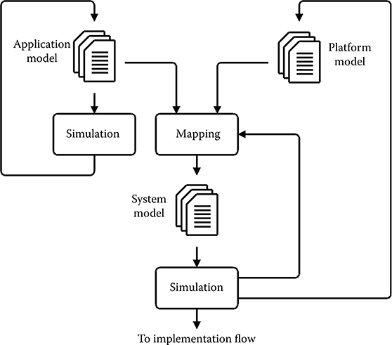
FIGURE 11.1 Overview of the presented system-level performance estimation framework.
The target architecture is modeled by a platform model that is composed of one or more service models. The service models of a platform model can be described at arbitrary levels of abstraction. In one extreme, they only associate a cost with the execution of a service, while on the other end of the spectrum, the service request is modeled in the platform model both cycle accurate and bit true. Costs can be associated with service requests irrespective of whether they are computed dynamically or precomputed. It is the cost of the execution of a service that differentiates various implementations of the particular service.
Quantitative performance estimation is performed at the system level through the simulation of a system model. A system model is constructed through an explicit mapping of the components of an application model onto the components of a platform model. The components of an application model, when executed, request the services offered by the component onto which they are mapped. This models the execution of the requested functionality, taking the implementation-specific details and required resources into consideration and associates a cost with each service requested. In this way, it becomes possible to associate a quantitative measure with a given system model and, hence, it becomes possible to compare systems and select the best-suited one from well-defined criteria.
11.1.3 Organization of the Chapter
The remaining part of this chapter is organized as follows: First an introduction to the modeling framework and its components is given followed by a small example of its use. Then, an extract of an industrial case study performed is presented and finally conclusions are given.
11.2 Service Models
A service model captures the functional behavior of a component through the notion of services. Services are used to represent the functionality offered by a given component without making any assumptions about the actual implementation. Concrete examples of services are functions of a software library, arithmetic operations offered by a hardware functional unit, or the instructions offered by a processor depending on the level of abstraction used to model the component.
The functionality offered by a service model, represented as services, can be requested by other service models through requests to the offered services. The detailed operation of a service model, that is, the implementation of the services offered, is hidden to other models. In that sense, a service model can be viewed as a black box component where the services offered are visible but not their implementation. Service models can be described at multiple levels of abstraction and need not be described at the same level to communicate. The clear separation of functionality and implementation through the concept of services implies that there is no distinction between hardware or software components seen from the point of view of the modeling framework. It is the cost associated with each service, which eventually dictates whether a component is modeling a hardware or software component.
A service model is composed of one or more service model interfaces and a service model implementation as illustrated in Figure 11.2. Interfaces are used to connect models, allowing models to communicate through the exchange of service requests. In this way, there is a clear separation of how behavior and communication of a component is described. The service model interfaces provide a uniform way of accessing the services offered and enabling service models to communicate and facilitate structural composition by specifying the sets of services that are offered and are required by the model. It is the active interfaces that specify required services and the passive interfaces that specify the offered services. In this way, structural composition is dictated by the interfaces that each service model implements and subsequently by the services offered and required. Only models fulfilling the required–provided service constraints can be connected. Although the interfaces dictate the rules of composition, the service model implementation is responsible for specifying the actual behavior of the service model. The specification implements the functionality of each of the services that are offered while optionally associating a cost with them.
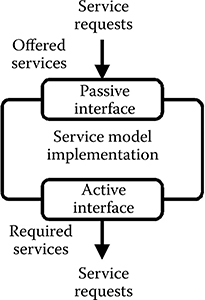
FIGURE 11.2 The service model basics.
The use of services allows a decoupling of the functionality and of the implementation of a component. In this fashion, several service models can offer the same service, implemented differently, however, and thus having different associated cost. In this way different implementations can be compared and evaluated based on a specific, preferred cost metric.
Intermodel communication is handled through service requests that have the benefit of allowing the initiator model to request one of the services specified, as required by the model, without knowing any details about the model that provides the required service or how it is implemented. When the service is requested, the service model providing the required service will execute the requested service according to the specification of the model. When the service has been executed, the initiator model is notified that the execution of the service requested has completed.
11.3 Service Model Interfaces
To facilitate structural composition of models and to allow communication between models, possibly described at different levels of abstraction, interfaces are used. The interfaces directly impose the rules of composition that specify how models can be connected by allowing only interfaces fulfilling the required–provided service constraints to be connected.
The use of interfaces also implies that multiple implementations of a service model can be constructed and be seamlessly interchanged, allowing different implementations to be investigated and described at different levels of abstraction, constrained only by the requirement that the service model implementations considered must implement the same interfaces.
Two types of interfaces are defined:
The passive service model interface specifies a set of services that the model implementing the interfaces offers to other models. The passive interface also includes structural elements allowing the interface to be connected to an active interface and provide means for requesting the services offered.
The active service model interface specifies a set of services that are required to be available for the model implementing the interface. The set of required services becomes available for the model that implements the active interface, when the active interface is connected to the passive interface of a service model, which offers a set of services in which the required set of services is a subset.
Active service model interfaces can only be connected to passive service model interfaces in which the set of services required by the active service model interface is a subset of the services offered by the passive service model interface. In essence, the composition rules, which specify which active service model interfaces can be connected to which passive service model interfaces, is dictated by the services required and services offered by the two connecting interfaces.
11.4 Service Requests
As mentioned briefly before, all intermodel communication is modeled using service requests exchanged via active–passive interface connections.
A service request can be viewed as a communication transaction between two components, similar to the concept of transaction-level modeling [11]. However, it is the implementation of the two service models that will determine if the service request will be implemented as a function call from, for example, a sequential executing piece of code to a function library or if it will be a bus transfer. Communication refinement is supported in several ways. Service requests can include arbitrary data structures as preferred by the designer of the model. If a communication channel must be modeled, an extra service model can be inserted between the two primary communicating service models as illustrated in Figure 11.3. The extra service model inserted will be transparent to the two communicating service models. This allows, for example, simple properties such as reliability of the communication channel to be modeled. More elaborate communication interconnects such as buses and network-on-chips can also be modeled.
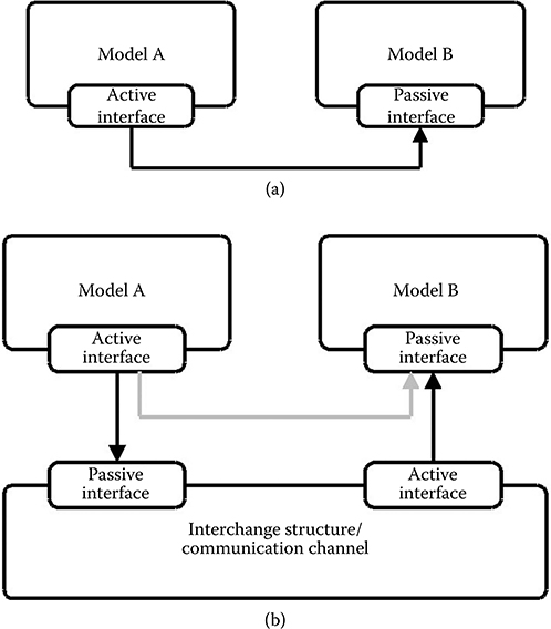
FIGURE 11.3 Intermodel communication. a) Model A is the active model, initiating communication with model B. b) The communication medium is now modeled explicitely using a separate service model.
A service request specifies the requested service, a list of arguments (which can be empty), and a unique request number used to identify the service request, for example, to annotate it with a cost. The argument list can be used to provide input arguments to the implementation of a service, for example, to allow modeling of dynamic dependencies or arithmetic operations on actual data values. Depending on the implementation of the service model, an arbitrary number of service requests can be processed in parallel, for example, modeling operating system schedulers, pipelines, very long instruction word, single instruction multiple data, and super scalar architectures.
A service request can be requested as either blocking or nonblocking. It is the designer of a model who determines whether a service request is requested as a blocking or a nonblocking request. The request of a blocking service request implies that the process of the source model that requested the service request is put into its blocked state until it has been executed, indicated by the destination model, as illustrated in Figure 11.4. A nonblocking service request, on the other hand, will be requested and the process of the source model, which requested the service request, will proceed—not waiting for the execution of the request to finish.
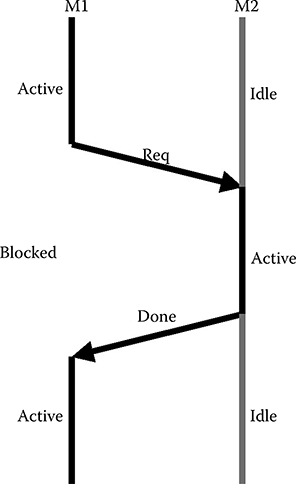
FIGURE 11.4 A process of model M1 requests a blocking service request from M2. M1 is blocked till the completion of the request.
A number of events are associated with a service request to notify the requester and receiver model of different phases of the lifetime of the service request. The lifetime and corresponding events of a service request are as follows:
The service request is being requested, indicated by a service request requested event.
The service request is being accepted for processing of the model by which it is requested, indicated by a service request accepted event.
The service request may be blocked, indicated by a service request blocked event.
The service request has been executed, indicated by a service request done event.
When a service request is being requested at a model interface, the receiver model has the possibility of receiving a notification to change its status to active. The requesting service model will similarly have the possibility of being notified when the request is accepted for processing in the receiver model (i.e., before the actual execution of the service request) and when it has finished executing the service request. During the evaluation of a service request, the request itself can become blocked because of one or more requirements not being fulfilled (e.g., because of mutually exclusive access to resources and missing availability of data operands). When a service request is being blocked during evaluation, the source model is notified to allow it to take appropriate actions, if any. However, the author of the requesting service model need not be interested in receiving these notifications and, hence, the model is allowed to ignore these. In this way, it is the designer who chooses event sensitivity for the individual processes of the service model implementation.
To handle multiple simultaneous service requests, the designer of a service model must incorporate a desired arbitration scheme. The arbitration scheme may be an integrated part of the model or it may be a separate service model itself. The latter is often advantageous if different arbitration schemes are to be investigated.
11.5 Service Model Implementations
To capture the behavior of a service model, the service model implementation must be defined. It is the service model implementation that captures the actual behavior of a service, possibly taking implementation-specific details into consideration. A service model must provide an implementation of all services offered by the passive interfaces implemented and optionally specify the latency, resource requirements, and cost of each service. There are no restrictions on how a service should be implemented. The abstract representation of the functionality, using services, implies that there is no immediate distinction between the representations of the hardware or software components. Whether a service model represents a hardware or software component is determined solely by its implementation and, eventually, its cost and thus an elegant unified modeling approach can be achieved.
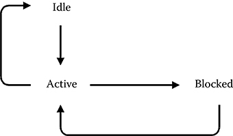
FIGURE 11.5 The possible states of a process of a service model.
11.5.1 Model-Of-Computation
To capture the implementation of a service model, concurrently executing processes are used as the general execution semantics. The service model implementation can contain one or more processes that each have the possibility of executing concurrently. A process executes sequentially and interprocess communication within a service model is done through events communicated via channels in which the order of events is preserved. All intermodel communication between processes residing in different service models is done using service requests via the service model interfaces defined by the model in which the processes reside.
A process can be in one of three states: idle, active, or blocked as shown in Figure 11.5, which also shows the valid transitions between the possible states. If a process is idle, it indicates that it is inactive but ready for execution upon activation. If a process is active, it is currently executing. If a process is blocked, it is currently waiting for a condition to become true and will not resume execution until this condition has been fulfilled.
To overcome the problem of finding a single golden model-of-computation for capturing all parts of an embedded system, the service model concept supports the existence of multiple different models-of-computation within the same model instance. Figure 11.6 shows an example of a system composed of service models, each described by a different model-of-computation. The service model concept allows these to coexist and communicate through well-defined communication semantics in the form of service requests being exchanged via active–passive interface connections.
Interesting work on supporting multiple different models-of-computation within a single model instance is presented in the theoretically well-founded tagged signal model [12] and the absent-event approach [13]. Both approaches show that it is possible to allow models-of-computation, defined within different domains, to be coupled together and allowed to coexist within the same model instance. In principle, the service model concept does not impose a particular model-of-computation. The individual models can be described using any preferred model-of-computation as long as communication between models is performed using service requests.
Currently, the focus of the framework is the modeling of the discrete elements of an embedded system only, that is, hardware and software parts, which can be represented by untimed, synchronous, or discrete event–based models-of-computation.
To synchronize models described using different models-of-computation and ensure a correct execution order, the underlying simulation engine is assumed to be based on a global notion of time that is distributed to all processes, no matter which model-of-computation is used. This contrasts with both the tagged signal model and the absent event approach. The former distributes time to the different processes through events, while the latter relies on the special absent event. The drawback of using a global notion of time is that processes cannot execute independently, which impacts simulation performance—it is very hard to parallelize such a simulation engine—the advantage, however, is that great expressiveness can be obtained in such a simulation engine. The simulation engine also tags all events with a simulation time value so that the event can be related to a particular point of simulation time, no matter which model-of-computation was used to describe the process that generated the event. However, this does not mean the individual service models must use this time tag and it is merely a practical requirement to schedule the execution order of the processes of the individual service models.
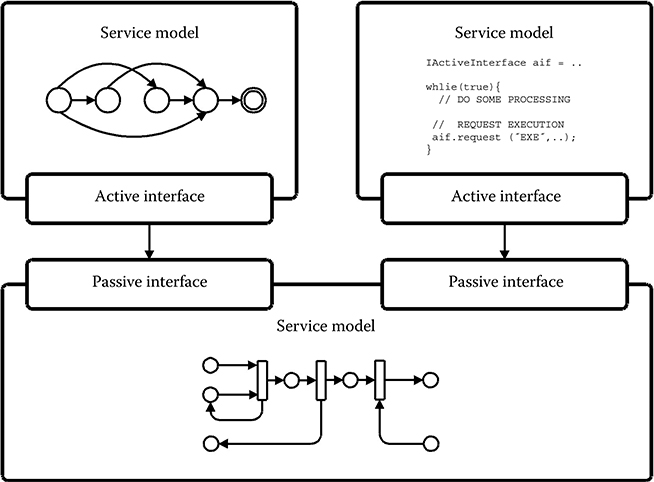
FIGURE 11.6 The service model concept provides support for heterogeneous models-of-computation to coexist.
Service models that have processes described using untimed models- of- computation obviously have no notion of time and perform computation and communication in zero time. This implies that a process of a service model that is described using an untimed model-of-computation is activated on the request of services offered by the model only (and not based on a specific point in time). The corresponding process then evaluates and produces possible outgoing service requests immediately.
Service models having processes described using synchronous models-of- computation do not use an explicit notion of time. Instead, a notion of time slots is used and each execution cycle lasts one time slot. In order for such models- of-computation to be used, the service model using a model-of-computation within this domain must specify the frequency of how often the processes of the model should be allowed to execute. The simulation engine will then ensure that the processes are evaluated at the specified frequency, in this way implicitly defining the actual time of the current time slot of the model.
Discrete-time models-of-computation are supported directly by the simulation engine, which provides a global notion of time that can be accessed from all processes. In this way, a process can describe behaviors that use timing information directly.
The generality of service models imposes few restrictions on the model-of- computation used to capture the behavior of the component being modeled. New models-of-computation can be added freely under the constraint that they must implement intermodel communication through the exchange of service requests and they must fit under the general execution semantics defined—that is, it must be possible to implement the preferred model-of-computation as one or more concurrently executing processes. It is the implementation of the service models that determines their actual behavior, and thus, it is the designer of the service model implementation who determines the model-of-computation used.
11.5.2 Composition
To tackle complexity, the service model concept supports both hierarchy and abstraction-level refinement. Here, the term abstraction-level refinement covers the process of going from a high level of abstraction to a lower level through gradual refinements of a given component, where a component may be replaced by a more detailed version (Figure 11.7).
This type of refinement is supported quite easily by the service model concept because of the fundamental property of the service model in which the functionality offered by a model is separated from the implementation. Two service models implementing the same set of interfaces, and thus offering the same set of services, can be freely interchanged, even though they differ in the level of detail used to model the functionality offered.
Furthermore, service models can be constructed hierarchically to investigate different implementations of a specific subpart of the model or to hide model complexity. One service model can be composed of several subservice models. However, it will then be only the interfaces implemented by the topmost model in the hierarchy that dictate which services are offered to other models. The hierarchical properties, combined with the use of interfaces, imply that designers who are using a model need only know the details of the interfaces implemented by the model and need not be concerned about the implementation details at lower levels in the model hierarchy.
To summarize, service models can be viewed as black-box components. The behavior of a service model is determined by the services requested via its active interfaces. The use of interfaces and service request, on the one hand, implies that there are no restrictions on the service model implementation, which is part of the service model that actually determines the behavior. This also implies that in principle there are no restrictions on which model-of-computation is used to describe the implementation of a service model.
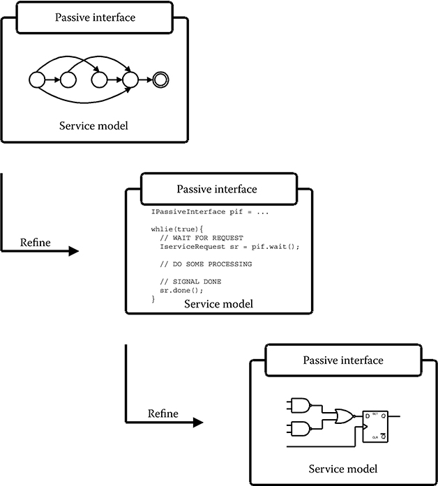
FIGURE 11.7 Abstraction-level refinement.
11.6 Application Modeling
Applications are represented by application models that are composed of an arbitrary number of components that can be executed in parallel. These executable components are referred to as tasks, each represented by a service model. Application models are used to capture the functional behavior and communication requirements of the application only. The tasks of an application model communicate through the exchange of service requests making communication explicit and implementation independent.
In the general case, a strict separation of the functional behavior, communication requirements, and implementation of an application must be applied in order for the application to be platform-independent. Thus, no assumptions on how the application is implemented should be made. However, in some cases, it may be desirable to include platform-specific information in the application model (e.g., in case an existing platform is modified) and, thus, support for including implementation-specific details in the application model is provided. However, including such detail will reduce the number of platforms onto which the application model can be mapped.
Application models can be executed and used for verifying the functional behavior of the model. However, at the application level of abstraction, there is no notion of time, resources, or other quantitative performance estimates. To obtain these, the service models of the application model must be mapped onto the service models of a platform model. When the tasks of an application model are mapped onto the processing elements of a platform model, the tasks, when executed, can request the services offered by the processing elements, modeling the execution of a particular functionality or set of functionalities.
11.7 Architecture Modeling
In contrast to the application models, the goal of the platform model is to capture a specific implementation of the functionality offered by the target architecture. In order for a platform model to be valid, it must offer all the services required by the application models that are mapped onto the platform. Several platform models can offer the same set of services, representing the same functionality, through different implementations. The differentiating factor will then be the cost associated with the execution of the applications on each of the candidate platforms.
The platform model of a given target architecture is implemented as a service model having one or more passive service model interfaces, as illustrated in Figure 11.8. Platform models are composed of an arbitrary number of service models, each modeling a component of the architecture, thereby forming a hierarchical model. The compositional properties of service models even allow multiple platform models to be merged into a single platform model. In this way, a modular approach can be taken in which subblocks of the target architecture are modeled and explored individually, if preferred.
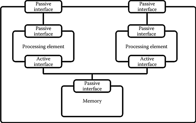
FIGURE 11.8 Illustration of a simple platform model consisting of two processing elements both connected to a block of shared memory.
The resulting set of services offered by a platform model is dictated by the composition of internal service models. From the tasks of the application models, which are mapped to the platform, the services of the platform model are accessible through the passive service model iinterfaces. This allows the tasks to request the services offered during simulation and so models the execution of the tasks.
The platform model also specifies how the service models, of which it is composed, are interconnected, thereby specifying the communication possibilities of the models. There are restrictions neither on how intercomponent communication is modeled, nor on the level of abstraction that is used. This implies that, in principle, all types of intercomponent communication methods are supported. In this way, platform models can represent arbitrary target architectures.
11.8 System Modeling
A system model is constructed by mapping the service models of one or more application models onto the service models of a platform model. If multiple service models from an application model are mapped onto the same service model of a platform model, a scheduler must be provided as part of the platform model. Schedulers are implemented as separate service models, for example, acting as abstract operating systems.
An application model is mapped onto a platform model by specifying how the active service model interfaces of an application model should be connected to the passive service model interfaces of the platform model. Mappings are specified in a separate XML file, which allows different mappings to be easily investigated without changing the actual model descriptions.
The service models of the platform model allow designers to associate quantitative cost with the execution of an application model. Without a platform model, the service models of an application model simply execute in zero time and have no cost associated. When the service models of an application model are mapped onto the service models of a platform model, it becomes possible to capture resource requirements, quantitative cost, and associate a time measure with the execution of the application model on the target platform. In this way, it is the platform model that introduces a notion of time into the simulations. Thus, the platform model orchestrates the execution of a given application model with respect to the timing and resource requirements defined by the individual parts of the application model that are executing on the platform model.
A given mapping is required to be valid in order for the resulting system model to be used for performance estimation through simulations. A mapping is said to be valid if and only if all the requested services of a given application model are offered by the processing elements of the platform model onto which it is mapped. However, it is not a requirement that all service models of an application model are mapped to the platform model. In the case where a service model of an application model is unmapped, only the functional behavior of the service model is modeled and no performance estimates are associated with that particular task. Currently, the validity of a given mapping is determined during runtime only, resulting in an error during simulation in the case of an invalid mapping. In the future, however, tools for performing such checks before runtime will be constructed. Also, future work will include the possibility of performing checks for the semantic validity of specific mappings to ensure, for example, that no deadlocks occur in a given mapping.
11.9 Simulation Engine
This section describes the simulation engine used for simulation of the models constructed in the presented system-level performance estimation framework with the objective to obtain quantitative performance estimates.
11.9.1 Discrete Event Simulation
To support multiple different models-of-computation, a discrete event simulation engine has been chosen for coordinating the execution of the individual service models and their internal processes. Discrete event modeling is used within a range of different application domains and described thoroughly in [14,15].
A custom simulation engine for prototype use supporting the modeling framework presented has been implemented during the course of this project. The reason for implementing a custom simulation was to obtain maximum control over the simulation kernel in order to be able to validate the ideas of the framework. The implemented discrete event simulation kernel keeps track of simulation time and schedules the execution of the individual processes of the service models according to their sensitivity to events.
As already described in Section 11.4, a number of events are associated with the lifetime of a service request, which by their occurrence can trigger processes sensitive to the event. The occurrence of a given event allows a waiting process to become activated at different phases of the simulation as described by the designer of the model and depending on the desired behavior.
The simulation engine provides basic semantics for expressing the behavior of a service model through a process-like behavior for modeling concurrency and a number of waitFor statements as listed in Table 11.1, which will cause the execution of the model to block.
waitFor(time) causes the process to block until the specified time has passed. The effect is that an event is being scheduled with a time tag of the current simulation time plus the specified time value. The simulation engine will fire the event when the specified simulation time has been reached and the process will resume its execution.
TABLE 11.1
Process Wait Types
waitFor(time) |
waitFor(service request, event type) |
waitFor(interface, service request type, event type) |
waitFor(event) |
waitFor(service request, event type) causes the process to block till the specified event type of the specific service request instance is being fired. When this occurs, the process will resume its execution and the time tag of the event will be decided by the simulation engine.
waitFor(interface, service request type, event type) causes the process to block till the specified service request type and event type is being fired at the specified service model interface. In this case, the simulation time will also be annotated by the simulation engine when the event is fired.
waitFor(event) causes the process to block till the specified event is fired. When the event is fired, the process will be notified and continue its execution.
11.9.2 Representation of Time
The simulation engine is implemented as a discrete event simulation engine using a delta-delay based representation of time [13]. The delta-delay based representation divides time into a two-level structure: regular time and delta-time. Between every regular time interval, there is a potentially infinite number of delta-time points t + δ, t + 2δ, …. Each event is marked with a time tag that holds a simulation time value, indicating when the event is to occur. Every time an event is fired and new events are generated having the same regular time value as the current time value of the simulation (e.g., in case of a feedback loop), the new event will have a time stamp with the same regular time value but now with a delta value incremented by one. The use of delta-delays ensures that no computations can take place in zero-time, but will always experience at minimum a delta-delay. The delta-delay based representation is making simulations deterministic because the use of delta-time makes it possible to distinguish between two events generated at the same point in time, which is to be processed first by looking at their delta-value.
Application models, on the one hand, have no notion of time. It is only when the application model is mapped onto a platform model that it becomes possible to annotate the execution time of the application model by relating the execution of its tasks and the generation of service requests to discrete time instances.
In the platform model, on the other hand, time is represented explicitly using the delta-based representation of time. Each model of the platform can be modeled with arbitrary delays or specify a clock frequency at which they want to be evaluated. In this way, it is possible to model synchronous components in the platform model, which are activated only at regular discrete time instances. Thus, the tasks of the application model are blocking while the service requests are being processed in the platform model, which enables associating an execution time metric with tasks. Similarly, it is possible to annotate tasks with other types of metrics such as power costs, etc.
A special event type is used to represent hardware clocks used for example by models described using clocked synchronous models-of-computation. These models do not use time explicitly, instead they represent time as a cycle count. To use synchronous models of computation in the currently implemented simulation engine, these models must specify a clock frequency that determines how often they are to be evaluated. Regular events are removed from the event list, executed, and then disposed. Because events are bound to a unique time instance, they can thus occur only once. The special event type used to represent hardware clocks, however, is implemented as a reschedulable event in the simulation engine, which takes care of handling the uniqueness of each instance of this event type. Such a clock event is automatically rescheduled and reinserted into the event list. Each clock event object has a list of active processes that are to be evaluated when the clock ticks. This list is updated dynamically during simulation, and in case a clock has no active processes in the active list, the clock itself is removed from the pending list of events to increase simulation performance. When a clock event object is inserted into the event list, it will be sorted according to the simulation time of the next clock tick of the clock event object. It is also possible to have a clock object that contains no static period. In this case, the clock ticks can be specified as random time points or as a list of periods that can be used once or repeated.
Of course, the platform model can also contain service models that are activated on the arrival of service requests only triggered by the event associated with the request of the service. In these cases, the occurrence of such an event, at a specific simulation time, will activate the blocking process. This blocking allows modeling of, for example, propagation delays associated with combinational hardware blocks, etc. The modeling of such elements can also be handled in zero regular time by means of the delta-delay mechanism.
11.9.3 Simulation
The simulation engine uses two event lists for controlling the simulation: one for delta events and one for regular events. The delta event list, on the one hand, contains only events with a time tag equal to the current simulation time plus one delta cycle. The regular event list, on the other hand, contains pending events with a time tag in which the regular time is greater than the current simulation time. The regular event list is sorted according to the time stamp of the events in increasing order. In this way, the head of the regular event list always points to the event with the lowest time tag.
The simulation engine always checks the delta event list first. If the list is not empty, the delta cycle count is incremented and all events contained in the delta event list are fired one by one till the list is empty, implying that all events belonging to the same delta cycle have been fired.
If no delta events are pending (i.e., the delta event list is empty), the simulation engine removes the first event in the regular event list and advances the simulation time to the time specified by the time tag of the event. Also, the current delta count is cleared and the event is then fired.
Delta-delay based discrete simulation engines suffer the risk of entering infinite loops where regular time is not advanced and only the delta cycle is incremented. A naive approach to handle this is implemented, allowing the designer to specify a maximum number of delta cycles to be allowed before the simulation engine quits the simulation.
The firing of an event can, of course, cause new events to be generated and scheduled in the simulation engine. If a new event is generated having its time tag set to the same regular time value as the current simulation time, it is added to the delta event list. Otherwise, it is scheduled according to its time tag and inserted into the regular event list according to the time tag specified. The delta event list contains only events with a time tag equal to the current simulation time plus one delta cycle.
After an event has been fired, it is checked if the event type of the event is periodic. Events belonging to a periodic event type (e.g., the special clock event object described in Section 11.9.2) are then automatically rescheduled and inserted into the event list at the correct position.
11.9.4 Service-Based Model-Of-Computation for Architecture Modeling
One example of a custom model-of-computation for describing service models is the model-of-computation developed for modeling synchronous hardware components presented in [16,17], which is based on Hierarchical Colored Petri Nets (HCPNs) [18]. HCPNs have been selected because of the great modeling capabilities with respect to concurrency and resource access and the compositional properties that match the requirements of service models well. Traditional HCPNs, however, suffer from a number of inadequacies with respect to model complexity and especially the obtainable simulation speed. These issues are addressed by, for example, defining special execution semantics. Details of the construction, simulation, and workings of service models based on HCPNs can be found in [16,17].
11.10 Producer–Consumer Example
To illustrate the use of the framework and elaborate on the different elements, a simple producer –consumer application is considered in the following.
The current implementation of the framework is in Java [19] and models are specified directly in Java as well through the use of a number of libraries developed for supporting the concept of service models, application models, platform models, and system models. In addition to the libraries, a simple graphical user interface has been implemented. The graphical user interface is built on the Eclipse [20] platform. It allows simulations to be controlled and inspected in a more convenient way than pure text-based simulations.
The first step to start using the presented framework is to construct an application model. The application model captures the functional behavior of the application in a number of tasks. It also specifies the communication requirements of the individual tasks explicitly, without any assumptions on the implementation, following the principle, on which the framework is founded, of separating the specification of functionality, communication, cost, and implementation. The application model serves as the functional reference in the refinement steps toward the final implementation. However, at this application level of abstraction, there is no notion of time or physical resources—hence only very rough performance estimates can be generated from a profiling of the application model.
Figure 11.9 shows an application model composed of a consumer task and a producer task, which communicate through an abstract buffer. Both the tasks and the abstract buffer are modeled by service models. The producer has an active interface that is connected to the passive write interface of the buffer offering a write service. Similarly, the consumer has an active interface that is connected to the passive read interface of the buffer model offering a read service. The producer and consumer models are the only active models, that is, only the producer and consumer models can initiate the request of services.
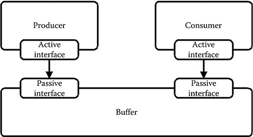
FIGURE 11.9 A simple application model consisting of a producer and a consumer communicating through an abstract buffer.
The service models are specified as one or more concurrently executing processes. Processes execute till they are blocked, waiting for some condition to become true. When the condition becomes true, the process can continue. Such behavior can be implemented using threads. The thread-context switching required, each time a process is being blocked or activated, has a high impact on simulation performance. Because we currently employ a global notion of time in the discrete event simulation engine, most processes will execute in a lock-step fashion. As a consequence, blocking and unblocking require frequent context switches. At the same time, threads provide more functionality than actually necessary now that only one process can be active at a time in the physical simulation engine. Thus, the desired behavior can be implemented in the much simpler concept of coroutines, which allows execution to be stopped and continued from the point where it was stopped. The current implementation of the simulation kernel thus uses a concept very similar to coroutines implemented in Java [19]. This requires that the designer of a process must divide the code body of the process into blocks. Blocks are executing sequentially and the execution of a block cannot be stopped. When the code contained in a block completes execution, the block returns a reference to the next block to be executed. In this way it is possible to model the blocking of a process on some condition and then when the condition becomes true, the process will resume its execution by executing the block of code returned by the previous executing block. Listing 11.1 shows the description of the main body of the producer service model.
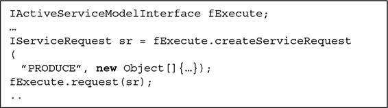
In this case a single process is used to capture the behavior of the producer. A similar description is made for the consumer which, however, is not shown. The main body of the producer is actually an infinite loop in which the producer first calculates some value, then instantiates a write service request with the calculated value as argument and then requests the write service via an active service model interface. It is possible to request a service and then continue the execution directly, however. In such a case, a waitFor statement is used to block the producer service model until the requested write service has been executed, signaled by the firing of a service-done event. When the service-done event is fired, the producer will be activated and rescheduled for execution in the simulation engine. The producer will then resume execution continuing from the point at which it was blocked.
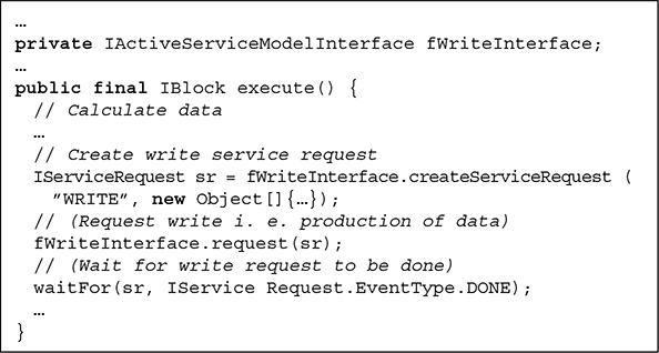
LISTING 11.1 Body of the producer service model main process.
As can be seen, the write service request is used for both signaling the request of a write service and for transporting the actual data values that are to be exchanged between the producer and buffer service model and that will be written into the buffer, eventually. In this way, arbitrary data and objects can be transferred.
The buffer model is activated only when a service request is requested through one of its passive interfaces. In such a case, the behavior of the read and write services depends on the implementation of the buffer. So, by simply interchanging the buffer model, different blocking or nonblocking read and write schemes can be conveniently investigated.
As an example, the buffer service model described in Listing 11.2 uses a blocking write policy.
Again, the main body is actually executing an infinite loop. The main body starts executing a waitFor statement, blocking the execution till the arrival of a write service request, indicated by the firing of a service request requested event of type write. In this case, the waitFor statement is not instance-sensitive as in the case of the producer, which was blocking for a service request done event on the instance of the requested write service request. Instead, it is blocking until a service request requested event of the specified type is fired, indicating a request through the active service model interface. This implies that whenever a service request requested event of type write is fired, the write process of the buffer service model will be scheduled for execution in the simulation engine and the write process will become active and continue its execution from the point at which it halted. It then starts the actual execution of the requested write service. If the buffer is already full, the write process will block once more until an empty slot in the buffer becomes available. Otherwise, the actual write to the buffer will be executed and a service request done event will be fired to notify the requester, in this case the producer, that the service request has been executed. A read process that implements a blocking read policy can be described analogously.
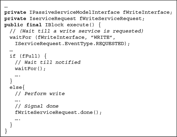
LISTING 11.2 Main body of the write process of the buffer service model.
To generate quantitative performance estimates, the task and buffer service models of the application model must be mapped to the service models of a platform model, which creates a system model. Performance estimates relevant for evaluating the different platform options can then be extracted from the simulation of the system model. When the service models of an application model are mapped to the service models of a platform model, the service models of the application model can, when executed, request the services offered by the platform service models. In this way, the functionality of, for example, a task, is represented by an arbitrary number of requests to services. When these requests are executed, they model the execution of a particular operation or set of operations. The execution of a service in the platform model can include the modeling of required resource accesses and latency only, or, depending on the level of abstraction used to describe the service model, even include the actual functionality including bit true operations.
The mapping of the service models of the application model to the service models of the platform model need not be complete, that is, it is allowed that only a subset of the service models of the application model are mapped.
In this case, the unmapped service models of the application model represent all functionality (i.e., both the control flow and data operations within the application model) and have no costs associated. In Figure 11.10, the consumer service model is an example of an unmapped service model.
On the other hand, the service model of the producer in Figure 11.10 is an example of a mapped task. As a first refinement step, the service model of the platform model, onto which the producer service model is mapped, is only used for latency modeling and for associating a cost with the execution of the producer. This is achieved by modeling a processing element that offers the service produce through a passive service model interface.
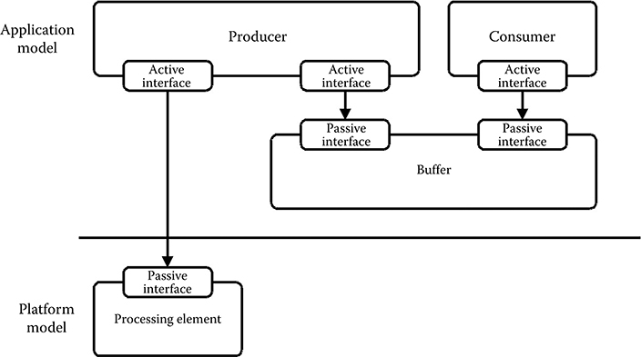
FIGURE 11.10 Only the producer task is mapped to the processing element of the platform model. The consumer task is unmapped and modeled functionally only.
LISTING 11.3 The refined production of data values, now depending on the platform model mapping.
The producer service model, as shown in Listing 11.3, then requests the produce service via its active service model interface during execution of the produce service, modeling a particular implementation in terms of cost and latency. In this example, the produce service is a very abstract service. In general, it is up to the designer to determine the level of abstraction used to associate with each service. One could also imagine the specification of required services for each arithmetic operation required to calculate the produced value. Currently, required services are specified manually, and to have a valid mapping of a service model from the application model onto the service model in a platform model, all required services must be provided by the service model of the platform model. The higher level of abstraction used to specify required services also implies that there are more options for mapping a model because the separation of functionality and implementation is retained.
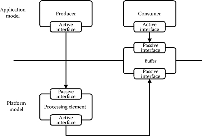
FIGURE 11.11 Only the producer task is mapped onto a processing element of the platform model. The consumer task is unmapped and modeled functionally only. Similarly, the FIFO buffer is only partially mapped, allowing it to be accessed from the active interface of the processing element in the platform model and at the same time be accessible from the active interface of the consumer task in the application model.
If preferred, it may also be possible to refine the processing element to include the calculation of actual data values. In this case, part of the behavior of the producer is modeled according to the functional specification in the application model, while another part is modeled according to a particular implementation in the platform model. As a result, different levels of abstractions are mixed seamlessly. This is particularly useful in the early stages of the design process where rough models of the platform may be constructed. In such a scenario, fast estimations of the effect of adding redundant hardware support for specific operations or even rough estimates of the effect of using multiprocessor systems, the effect of buffer sizes, etc. can be explored. This scenario may be refined to a level where cycle accurate and bit true models are described, but still leaving the control flow of the application to be handled in the application model and modeling only the cost of control operations in the platform model.
Such an example is seen in Figure 11.11, where the producer task could be implementing, for example, loop control in the application model directly. At the same time, it only implements part of the functionality of the loop body through requests to services offered by the service model of the processing element in the platform model onto which it is mapped. Figure 11.11 also shows how it is possible for the producer, mapped to and executing on the processing element, to communicate through a partially mapped buffer with the functional consumer service model, which is modeled only in the application model.
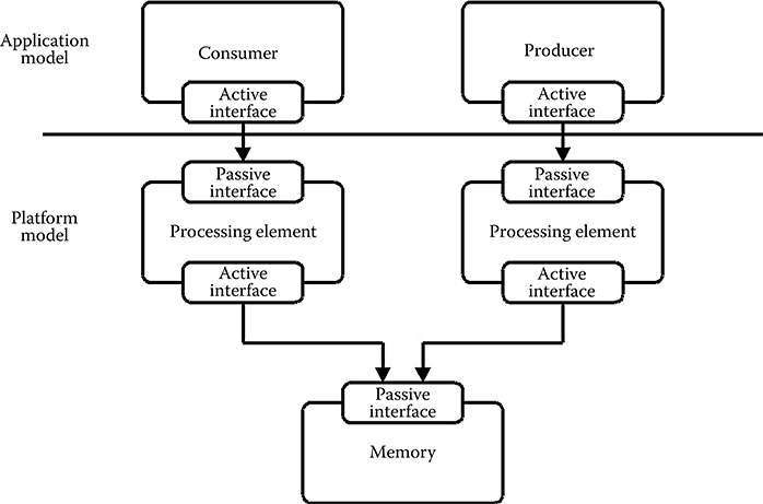
FIGURE 11.12 Both the producer and consumer tasks are now mapped onto processing elements of the platform model. The FIFO buffer is mapped to the service model, modeling a block of shared memory to which both processing elements have access.
Finally, as shown in Figure 11.12, it is possible to model a full mapping of an application model onto a platform model, including both the active service models, in this case the producer and consumer running on one or more processing elements, and the passive service models, in this case the buffer mapped onto a block of memory. Still, it is possible to mix partially functional behavior modeled in the application model with the actual behavior of the implementation modeled in the platform model. In the most extreme case, the producer and consumer is represented solely by a set of requests to the services offered by the processing element of the platform model onto which it is mapped. In this case, the complete functionality is modeled in the platform model. Consequently, the complete task is represented by a service request image, directly equivalent to a binary application image of a processor. Another advantage of the support for such compiled tasks is that a platform model described at this level of abstraction can also be used for performance estimation of compiler technologies.
It is important to notice that service models described at different levels of abstraction can be mixed freely, providing great expressiveness and flexibility. Thus, depending on the level of abstraction used to describe the service models of a platform model, the execution of a requested service can model the actual functionality of the target architecture. Furthermore, the required resources and cost in terms of, for example, latency or power of the service can be included. Thereby, the functionality of the application model mapped onto the platform model is modeled according to the actual implementation, including, for example, the correct bit widths and availability of resources, simply by refining the platform model without changing the application model. It then becomes possible to annotate a given task in the application model with the cost of execution. This then adds a quantitative cost measure for use in the assessment of the platform.
11.11 An Industrial Case Study
As an illustration of the usage of the presented framework, an extract of the industrial case study presented in Tranberg-Hansen et al. [21] is given, in which a mobile audio processing platform developed by the Danish company Bang & Olufsen ICEpower was explored.
11.11.1 A Mobile Audio Processing Platform
The mobile audio processing platform, illustrated in Figure 11.13, is comprised of a digital front end and a class D amplifier including the analog power stage on-chip. The platform offers stereo speaker and stereo headphone audio processing, resulting in a total of four audio channels being processed.
The application receives one common stereo audio stream, consisting of a left and right audio stream. After the processing of algorithm A, these are split into four separate audio streams. Two are for speakers and two are for headphones, to allow a separate processing of the speaker and the headphone streams. The resulting application model is shown in Figure 11.14.
The platforms considered here are based on the use of an application-specific instruction set processor (ASIP), which is optimized to execute the type of algorithms necessary in the case-study application. The ASIP has a shallow three-stage pipeline and offers 61 different instructions. Even though the pipeline is shallow, the instructions are relatively complex: the processor offers a dedicated second-order IIR filter instruction that is used heavily in the application considered. Two versions of the ASIP were described: (1) a high-level model that models only the latency of each instruction offered and (2) a detailed cycle accurate and bit true model. The latency models do not model the actual functionality but only the resource access and latency of each service without any modeling of data dependencies.
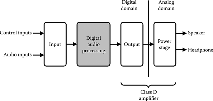
FIGURE 11.13 Overview of the case-study platform.
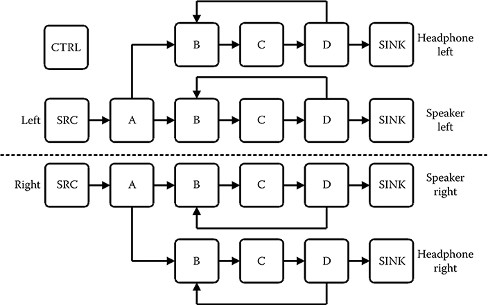
FIGURE 11.14 The application model of the case study. The application model contains 14 tasks (2 × A, 4 × B, 4 × C, 4 × D) for modeling the processing of the audio streams, 6 tasks (2 × SRC, 4 × SINK) for modeling the audio interfaces to and from the environment, as well as the environment itself, and finally an additional task (CTRL) for modeling the changes of the application state and/or control parameter changes that influence the individual audio processing parts.
A number of platform models were constructed consisting of one to four ASIPs (ASIPx1-ASIPx4). Subsequently, the application model, capturing the functional requirements of the application, was mapped onto the platform models based on the latency ASIP service models. Because the latency-based service models do not model the actual functionality, the control flow of the application must be handled in the application model and the tasks mapped to the individual latency-based service models. This group of system models is hence named latency. The four platforms were then refined to use the bit true and cycle accurate service model of the ASIP using the compositional properties of the framework. The tasks of the application models were mapped to the ASIP service model processing elements. The tasks were represented as service request images generated using the existing compiler infrastructure associated with the ASIP. In this way, a one-to-one correspondence with the physical execution of the application can be obtained. These system models are referred to as compiled system models.
To relate the simulation speed and quality of the performance estimates produced by the models described using the modified HCPN model-of-computation, a register transfer level implementation of the ASIPx1 platform was created in the hardware description language Verilog, referred to as the RTL model in the following.
TABLE 11.2
Estimated Number of Cycles for the Processing of 3000 Samples In One Audio Channel at Three Levels of Abstraction. A, B, C, and D are The Different Tasks of the Application Being Executed
|
Latency |
Compiled |
Rtl |
A |
84,034 |
102,034 |
102,034 |
B |
123,041 |
129,384 |
129,384 |
C |
33,011 |
33,011 |
33,011 |
D |
153,051 |
168,056 |
168,056 |
Total |
393,137 |
429,143 |
429,143 |
11.11.2 Accuracy
The simulations performed, using the RTL model, were compared with the results obtained from the performance estimation framework.
Table 11.2 shows the estimated number of cycles used to process a stereo audio channel produced by the framework for the latency and the compiled ASIPx1-system model and estimates extracted from the RTL model simulations. The table shows that the cycle estimates obtained from the latency model in which only the latency-based service models are used is not cycle accurate. The cycle estimates produced by the latency model are, in general, too optimistic. This is caused by the fact that the latency-based model does not take data dependencies into account. In the other range of the scale, in terms of accuracy, the table also shows the cycle estimates of the refined compiled model in which a cycle accurate and bit true modeling of the components was used. In this case, the cycle estimates are identical with the estimates obtained from the RTL model as can be seen from the table.
The RTL model constructed was also used to make a comparison of the functional results produced by the framework using the compiled version of the ASIPx1 platform, which proved to be 100% identical to the results obtained from the RTL model. Furthermore, the time required to describe the model using the presented framework is much less than the time required to describe the equivalent RTL model because of the higher level of abstraction used. More importantly, it is significantly faster to modify a model of the framework in case of bug fixes or functionality extensions.
11.11.3 Simulation Speed
Table 11.3 shows the measured simulation speeds expressed as cycles per second for the individual system models investigated. Simulations were performed on a 2.0 GHz Intel Core 2 Duo processor with 2 GB RAM. What is most interesting is the substantial speedup seen when comparing the simulation speed of a detailed bit true and cycle accurate version of the ASIPx1-system model as opposed to the equivalent regi ster transfer level simulation. The ASIPx1-system model runs at approximately 20 million cycles per second with all algorithms enabled, including data logging, and the functionally equivalent RTL description runs with approximately 15,000 cycles/second resulting in a speedup of more than 1000× compared to the RTL simulation.
TABLE 11.3
Obtainable Simulation Speed (Simulation Cycles Per Second) Of The Investigated System Models
|
Latency |
Compiled |
Rtl |
ASIPx1 |
21.7M |
19.9M |
15,324 |
ASIPx2 |
18.6M |
15.8M |
N/A |
ASIPx3 |
17.2M |
13.8M |
N/A |
ASIPx4 |
15.9M |
12.4M |
N/A |
11.12 Conclusion
This chapter has introduced a novel compositional modeling framework for system-level performance estimation of heterogeneous embedded systems. The framework is simulation-based and allows performance estimation to be carried out throughout all design phases ranging from early functional to cycle accurate models. Using a separation of the specification of functionality, communication, cost, and implementation, combined with an interface-based approach, provides a very flexible framework with great refinement possibilities. Also, the framework enables the possibility for components, described at different levels of abstraction, to coexist and communicate within the same model instance.
Acknowledgments
The authors acknowledge the industrial case provided by the DaNES partner Bang & Olufsen ICEpower A/S.
The work presented in this chapter has been supported by DaNES (Danish National Advanced Technology Foundation), ASAM (ARTEMIS JU Grant No 100265), and ArtistDesign (FP7 NoE No 214373).
References
1. Benini, Luca, Davide Bertozzi, Alessandro Bogliolo, Francesco Menichelli, and Mauro Olivieri. 2005. “Mparm: Exploring the Multi-Processor SoC Design Space with SystemC.” The Journal of VLSI Signal Processing-Systems for Signal, Image, and Video Technology 41 (2): 169–82.
2. Cesario, W. O., D. Lyonnard, G. Nicolescu, Y. Paviot, Sungjoo Yoo, A.A. Jerraya, L. Gauthier, and M. Diaz-Nava. 2002. “Multiprocessor SoC Platforms: A Component-Based Design Approach.” IEEE Design and Test of Computers 19 (6): 52–63.
3. Gao, Lei, K. Karuri, S. Kraemer, R. Leupers, G. Ascheid, and H. Meyr. 2008. “Multiprocessor Performance Estimation Using Hybrid Simulation.” 2008 45th ACM/ IEEE Design Automation Conference, 325–330.
4. Kunzli, S., F. Poletti, L. Benini, and L. Thiele. 2006. “Combining Simulation and Formal Methods for System-Level Performance Analysis.” Proceedings of the Design Automation & Test in Europe Conference 1: 1–6.
5. Mahadevan, Shankar, Kashif Virk, and Jan Madsen. “Arts: A SystemC-Based Framework for Multiprocessor Systems-on-Chip Modelling.” Design Automation for Embedded Systems 11 (4): 285–311.
6. Pimentel, A. D., C. Erbas, and S. Polstra. “A Systematic Approach to Exploring Embedded System Architectures at Multiple Abstraction Levels.” IEEE Transactions on Computers 55 (2): 99–112.
7. Tranberg-Hansen, Anders Sejer, and Jan Madsen. “A Compositional Modelling Framework for Exploring MPSoC Systems.” In CODES+ISSS ’09: Proceedings of the 7th IEEE/ACM International Conference on Hardware/Software Codesign and System Synthesis, 1–10. New York, NY, USA: ACM.
8. Keutzer, K., A. R. Newton, J. M. Rabaey, and A. Sangiovanni-Vincentelli. 2000. “System-Level Design: Orthogonalization of Concerns and Platform-Based Design.” IEEE Transactions on Computer-Aided Design of Integrated Circuits and Systems 19 (12): 1523–43.
9. Balarin, Felice, Massimiliano Chiodo, Paolo Giusto, Harry Hsieh, Attila Jurecska, Luciano Lavagno, Claudio Passerone et al. 1997. Hardware-Software Co-Design of Embedded Systems: The POLIS Approach. Norwell, MA, USA: Kluwer Academic Publishers.
10. Kienhuis, B., E. Deprettere, K. Vissers, and P. Van Der Wolf. 1997. “An Approach for Quantitative Analysis of Application-Specific Dataflow Architectures.” In ASAP ’97: Proceedings IEEE International Conference on Application-Specific Systems, Architectures and Processors, pp. 338–349.
11. Cai, L. and D. Gajski. 2003. Transaction Level Modeling: An Overview. In CODES+ISSS ’03: Proceedings of the 1st IEEE/ACM/IFIP international conference on Hardware/software codesign and system synthesis, pp. 19–24.
12. Lee, E. A. and A. Sangiovanni-Vincentelli. 1998. “A Framework for Comparing Models of Computation.” Computer-Aided Design of Integrated Circuits and Systems, IEEE Transactions on 17 (12): 1217–29.
13. Jantsch, Axel. 2003. Modeling Embedded Systems and SoCs—Concurrency and Time in Models of Computation. Morgan Kaufmann Burlington, MA: Systems on Silicon.
14. Cassandras, Christos G. 1993. Discrete Event Systems: Modeling and Performance Analysis. Aksen Associates, Inc., Homewood, IL.
15. Wainer, G. A. and P. J. Mosterman. Discrete Event Simulation and Modeling: Theory and Applications. Computational Analysis, Synthesis, and Design Of Dynamic Systems Series. CRC Press, Taylor and Francis Group, 2010.
16. Tranberg-Hansen, Anders Sejer, and Jan Madsen. 2008. “A Service Based Component Model for Composing and Exploring MPSoC Platforms.” In ISABEL ’08: Proceedings of the First IEEE International Symposium on Applied Sciences in Bio-Medical and Communication Technologies, pp. 1–5.
17. Tranberg-Hansen, Anders Sejer, Jan Madsen, and Bjorn Sand Jensen. A Service Based Estimation Method for MPSoC Performance Modelling. In Proceedings of the International Symposium on Industrial Embedded Systems, SIES 2008, pp. 43–50.
18. Jensen, Kurt. 1992. Coloured Petri Nets. Basic Concepts, Analysis Methods and Practical Use. Volume 1, Basic Concepts. Springer-Verlag Germany.
19. Sun Mircrosystems. Java SE 1.6, 2008. http://www.java.sun.com.
20. Eclipse Foundation. Eclipse. http://www.eclipse.org/.
21. Tranberg-Hansen, Anders Sejer, and Jan Madsen. 2009. “Exploration of a Digital Audio Processing Platform Using a Compositional System Level Performance Estimation Framework.” 2009 IEEE International Symposium on Industrial Embedded Systems, SIES ’09, pp. 54–7.