Chapter 19 Real-Time Simulation Platform for Controller Design, Test, and Redesign

Control is a problem of finding a suitable (control) input driving a given system to a desired behavior. In general, there is extensive literature introducing the field of control and providing background material on solving control problems [1–3]. Having a system displaying a desired behavior is usually achieved by designing a controller that produces the necessary control in terms of the fed back actual (plant) output and a reference signal representing the desired (plant) output. The design of a controller working well for a given real plant in an actual environment requires the consideration of the behavior of the actual plant under the actual operating conditions [4–11]. In one extreme, such a controller design problem can be attempted to be solved by examining the simulated controller on a simulated plant under simulated operating conditions [2,12], while in another extreme, the approach relies on testing and tuning the controller hardware on the physical plant in the actual environment [13,14]. Testing the proposed controllers’ performance on the simulated or physical plant is followed by a redesigning or parameter tuning process performed offline or online. Both approaches have their own advantages/disadvantages and also difficulties for experimentation. For most of the cases, examining the controller candidates directly on the physical plant may not be possible in the laboratory environment or may be dangerous because of possible damages that may result [15,16]. In between these extremes lies an approach that mimics the physical plant in real time and in actual environmental conditions, especially in combination with the analog/ digital interface units. However, such an approach is not only complicated in software simulations but it also yields, with great probability, unreliable simulators that are highly sensitive to the unavoidable modeling errors that each simulated unit embodies [17,18].

In spite of these drawbacks, in general, simulation of control systems is preferred (1) for understanding the behavior of the plant together with its actuator and sensory devices based on their identified models obtained before an expensive and belabored implementation (i.e., for analysis) and (2) for testing the designed controllers whether the design specification are met (i.e., for synthesis). Analysis and/or synthesis platforms developed for general and also for certain specific purposes are documented in other works [16–27]. In the controller synthesis case, which is the main concern in this chapter, testing the controllers is followed by a redesign and/or tuning procedure. The developed controller design–test–redesign platform (CDTRP) consists of a simulator together with a software manager on a personal computer (PC) that is implemented with a graphical user interface (GUI), a microcontroller based emulator, and a hardware peripheral unit. CDTRP is intended to have the advantages of using simulated or emulated plants in the controller design and also of testing the candidate (simulated, emulated, or actual) controllers on the almost actual operating conditions.

Depending on the implementation of the controller, plant, and peripheral unit as simulation, emulation, or physical hardware, the developed CDTRP can be operated in 24 different real-time operation modes (Tables 19.1 through 19.3). These operation modes are also referred to as real-time simulation modes [19–27], meaning the samething throughout this chapter. The simulator and emulator in all the 24 modes of CDTRP are designed for performing real-time simulations; however, they can be run faster or slower for different purposes. For example, a fast running plant emulator or simulator can be used for model reference adaptive control. So, the simulation modes that can be realized in the platform are not restricted to the mentioned 24 real-time modes. Some of the real-time simulation modes correspond to the well-known “hardware- in-the-loop simulation” [19–27], where the controller is realized as hardware and the plant is implemented on the PC or in the emulator (Tables 19.1 through 19.3). Some of the other modes correspond to the well-known “control prototyping” and “software-in-the-loop simulation” [19, 20]. Both simulate the controller on the PC but differ from each other in the plant part. The first one is the physical and the second is implemented on the PC (Tables 19.1 through 19.3). The simulation modes of the developed CDTRP include not only the abovementioned “hardware-in-the-loop simulation,” “control prototyping,” and “software-in-the-loop simulation,” but also, up to the knowledge of the authors, all the other simulation modes in the literature.

TABLE 19.1
Taxonomy of Real-Time Simulation Modes of CDTRP. The Peripheral Unit Is Implemented in the Simulator (PC)

Plant Controller	Simulator (In Pc)	Emulator	Physical (Hardware)
Simulator (in PC)	S-S-S	S-E-S	S-P-S
Emulator	E-S-S	E-E-S	E-P-S
Physical (Hardware)	P-S-S	P-E-S	P-P-S

TABLE 19.2
Taxonomy of Real-Time Simulation Modes of CDRTP. The Peripheral Unit Is Implemented in the Emulator

Plant Controller	Simulator (In PC)	Emulator	Physical (Hardware)
Simulator (in PC)	S-S-E	S-E-E	S-R-E
Emulator	E-S-E	E-E-E	E-P-E
Physical (Hardware)	P-S-E	P-E-E	P-P-E

TABLE 19.3
Taxonomy of Real-Time Simulation Modes of CDRTP. The Peripheral Unit Is Implemented as Physical Hardware

Physical (Hardware)	Simulator (In Pc)	Emulator	Physical (Hardware)
Simulator (in PC)	–	S-E-P	S-P-P
Emulator	–	E-E-P	E-P-P
Physical (Hardware)	–	P-E-P	P-P-P

Note: The first column modes are realized in CDTRP without using an additional analog interface extenstion for the PC.

The CDTRP platform is developed according to a controller design–test–redesign methodology, which can be stated as follows:

To provide a high level of flexibility of choosing and testing controller and plant models from a wide variety by the simulator unit in the early stages of the controller design.
To create environmental conditions as close as possible to the real world by the emulator and peripheral units in the final stage of the controller design process.

So, the CDTRP can be used for the following:

The design–test–redesign of the controllers under the framework of a chosen specific controller design method (such as an adaptive or robust method)
Comparison of the performances of the different controller design methods, techniques, and algorithms on the simulated, emulated, or physical plants with the emphasis of the controller design in real time and the actual environment, and so supporting the selection of the best controller for a specific applications, on the other hand serving as a test-bed for researchers in examining their immature controller design method in its development phase
Verification and validation of a plant model [28–31] based on the simulated and emulated plants with emphasis on running in real time and in the actual environment
Controller design requiring a parameter training procedure based on the measurements and also calculations on an emulated (identified) plant model as in done artificial neural networks–based controller design methods [24,32–35]
Low cost real-time implementation of control systems based on the benchmark plants that are of educational value but difficult or impossible to realize in an educational laboratory [36]

Similar real-time simulation platforms have been realized in the literature [6,10, 11,21,22,37,38]; however,

They are not dedicated to being a general purpose design–test–redesign controller platform.
They are restricted either to a specific control application (e.g., robot, specific electrical motors, pantograph, or dynamometer) or to a certain type of simulation mode such as software-in-the-loop or hardware-in-the-loop.
None of them possesses a (physical) hardware peripheral unit that comprises all of the (actual) analog and digital actuators, sensory devices, the external disturbance, parameter perturbation signal derivers, and analog/digital controller hardware components, and so they have the ability to recreate an actual environment in a more restricted sense than the CDTRP.
The frequency limits for the real-time simulation modes realized by these platforms have not been reported in contrast to the CDTRP.
They do not have a GUI unit capable of monitoring and controlling the overall simulation platform such as the one that the CDTRP includes.

This chapter is organized as follows. In Section 19.2, the developed platform CDTRP is briefly described presenting its subunits (i.e., the emulator card, the software simulator on the PC, the hardware peripheral unit, and the GUI managing the overall platform). Structural properties and functions of the emulator, simulator, and peripheral unit; the facilities supplied by the GUI; and a block diagram for the emulator card that is made up of the PIC microcontroller and its input–output interfaces are given in this section. The real-time operating modes provided by the CDTRP are described in Section 19.3 by the introduced taxonomy together with a soft categorization based on their suitability to the design, test, and redesign stages in a controller design process in Section 19.4. The implementation of a plant emulator card and experimental setup of the developed CDTRP are given in Sections 19.5 and 19.6. In Section 19.7.1, the implementation of the operating modes of the CDTRP are demonstrated on several benchmark plants for, in a sense, verification of the simulation platform. The experimental results on the implementation of design–test– redesign procedure of a physical plant (i.e., a micro DC motor) are given in Section 19.7.2. In Section 19.7.3, the coupled Lorenz chaotic systems and pendulums are used as tools for investigating the frequency range for the plant and controller dynamics to be simulated and/or emulated reliably in different real-time operating modes of the CDTRP. The conclusions of the developed CDTRP are given in Section 19.8.

19.2 Structure and Functions of the CDTRP

The CDTRP comprises four main units, which are a real-time simulator running on a PC, a real-time plant emulator realized in a plant emulator card, a hardware peripheral unit for recreating a physical environment for the plant emulator, and a GUI on the PC that manages the entire platform. The structure and the interconnection of the subunits of CDTRP are depicted in Figure 19.1. The first unit is the software simulator implemented on the PC. It aims to simulate the controller, the plant, and/or the peripheral unit components depending on the operating modes of the platform (i.e., it simulates, for instance, the plant if it is active in the chosen mode of operation). The simulation program consists of MATLAB^® 7.04 code and it requires the controller algorithm and plant model as MATLAB code. The simulator is designed to run essentially in real time; however, it can run in any time step faster or slower than real time, which may be preferred depending on the application.

The second unit is the plant emulator card whose core is the PIC microcontroller 18F452. The microcontroller is devoted to emulate the controller, the plant, and/or the peripheral unit components depending on the operating modes of the platform. The plant emulator card also possesses digital and analog interfaces for the communication of the plant emulator with the other units of CDTRP (i.e., the GUI and the hardware peripheral unit card). The PIC is programmed by Custom Computer Services C Program Compiler Version 4.084 software run on the PC before installing it on the plant emulator card, which allows the PIC software to be managed by the GUI and to communicate with the PC and the hardware peripheral unit card. Note that the details on the hardware realization of the emulator card are given in Section 19.5.

The third unit of the CDTRP, that is, the hardware peripheral unit card, is the most flexible part of the platform: depending on the application, it contains a (analog and/or digital) hardware controller, actuators, sensory devices, and signal drivers corresponding to the external disturbance and parameter perturbations to recreate the physical environmental conditions for the plant emulator.

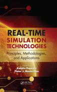
The fourth unit of the CDTRP, the GUI, provides the management of the entire platform. The GUI is implemented with more than 2000 lines of MATLAB code in the MATLAB GUI designer tool. The GUI serves as a monitoring and controlling unit for the platform. The GUI manages all operating modes listed in Tables 19.1 through 19.3 and the environmental conditions provided by the hardware peripheral card. A view of the front panel of the GUI is given in Figure 19.2 where the monitoring and controlling tools supplied to the users by the GUI are visible. The main features and management (i.e., monitoring and controlling) facilities of the GUI are presented in more detail in other work [39].

Images

FIGURE 19.1 Structure of controller design–test–redesign platform.

Images

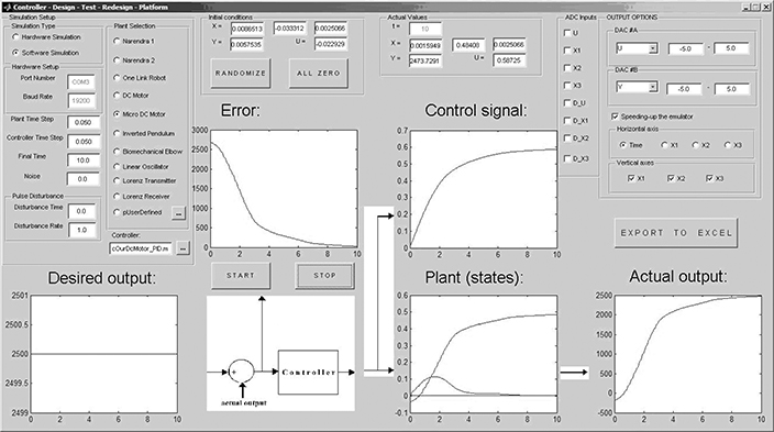
FIGURE 19.2 Front panel of the graphical user interface for the platform.

19.3 Taxonomy of Real-Time Simulation Modes Realized by CDTRP

With the features of the GUI mentioned in Section 19.2, the developed simulation platform CDRTP becomes self-contained and it can implement 24 different real-time operating modes given in Tables 19.1 through 19.3.

The operating modes given in Tables 19.1 through 19.3 are obtained depending on the implementation of controller, plant, and peripheral unit as the simulator (PC), emulator, or physical (analog/digital) hardware. Other than S-S-S, E-E-E, and R-R-R modes, all modes will be called as mixed modes since at least two of the controller, plant, and peripheral unit are implemented in different units of CDTRP (i.e., the simulator (PC), the emulator, and the physical hardware). Note that the controllers are applied to the plants within the unity feedback gain configuration in all modes. However, the modes are by no means restricted to this particular (yet quite general) feedback configuration, which means the other possible configurations can be created by making some modifications to the introduced GUI. The simulator and emulator of CDRTP can be run faster than real time or run without hard time limits. However, these cases (mentioned in Isermann [19]) are beyond consideration in the presented work, since the focus is on test and design of controllers under the criterion of working well for real-time operations.

The first column modes in Table 19.3 cannot be realized in CDTRP without using an analog interface feeding the output of the physical peripheral unit to the PC where the plant is simulated.* The actuator, sensors, disturbance, and parameter perturbation effects that are created in the peripheral unit using analog/digital hardware can be embedded in the emulator by means of the emulator interface. So, the S-E-R, E-E-R, and R-E-R modes of CDTRP constitute a contribution to the real-time simulation literature, since there is no such interface possibility of the simulators running on PCs and the available emulators in the literature.

R-R-R operating mode corresponds to an actual control system and not a simulation mode. S-S-S mode where all parts of the control system are simulated on a PC is the most commonly used mode in the literature so that many software tools are available. All the real-time S-S-S, S-E-S, E-S-S, E-E-S, S-S-E, S-E-E, E-S-E, and E-E-E operating modes where the controller, plant, and peripheral unit are all implemented in the simulator (PC), or possibly in the emulator, would be considered the so-called “software-in-the-loop” simulation in the literature [19, 20]. In a similar way, the modes S-R-S, E-R-S, R-R-S, S-R-E, E-R-E, S-R-R, and E-R-R where the plant under test is physical would be considered the so-called “prototyping modes” [19] and the modes R-S-S, R-E-S, R-S-E, R-E-E, and R-R-E where the controller is implemented as physical hardware while the plant is simulated would be considered the so-called “hardware-in-the-loop” simulation [19–27]. It should be noted that giving a single name for different modes is confusing, and so it may be better to use the three-letter based index provided in Tables 19.1 through 19.3 to distinguish different modes. An alternative may be the separation of the modes into subclasses such as simulated-controller, simulated-plant, simulated-peripheral, emulated- controller, emulated-plant, emulated-peripheral, physical-controller, physical-plant, or physical-peripheral classes of modes. Each of these modes then refers to a set of modes whose common property is specified by the class name, for example, the real-plant class consists of all modes where the plant is real but the controller and peripheral may be simulated, emulated, or physical. Throughout the chapter, three-letter indices will be used for the individual modes and the lastly mentioned classes will be used for the associated set of modes whenever appropriate.

In a further refinement, the set of operating modes can be extended by assigning extra letters for each element of peripheral subunit, that is, actuator, sensor, disturbance, and perturbation, depending on their implementation in simulator or emulator or as physical hardware. A hardware realization for controllers and components of the peripheral unit is application specific. In other words, depending on the application, the hardware may be a fully analog system (as in the chaotic synchronization application presented in Section 19.7.3) or a microcontroller or digital signal processor card equipped with analog interface to communicate with the emulated or physical plant.

19.4 Categorization of Cdtrp Modes Based on Their Suitability for Design, Test, and Redesign Stages

According to the main issue addressed, which is to design controllers that achieve high performance at the physical plant under actual environmental conditions, a controller design procedure following a three stage path is proposed.

* Of course, such an extension is possible but at the expense of additional cost.

(Initial) Design Stage: Use a simulation mode of CDTRP that enables implementing any kind of controller, plant, and peripheral components with a relatively much higher memory and speed provided by CPU as compared to the PIC processor and with a high flexibility of changing the models and parameters of controller, plant, and peripheral components in an efficient way. Of course, the most suitable mode for the initial design stage is S-S-S. Depending on the control application, on the chosen (initial) set of candidate control methods, and also on the experience and knowledge of the control system designer, the modes listed in the first rows and columns of Tables 19.1 through 19.3 are typically preferred in the initial design stage.

Test Stage: Use an operating mode of CDTRP that examines the control methods in terms of their performances under conditions as close as possible to the physical world and so provides a tool for eliminating the controller candidates that give poor performances on the physical plant in the actual environment. In other words, the modes suitable for the test stage are the ones that provide physical performance features, providing sufficient information to make a correct decision on their usability in deployed applications. All these modes provide a flexible implementation efficiency with the ability to create and change the models and their parameters for controller, plant, and peripheral components, though, of course, to a lesser extent as compared to the initial design stage. In this sense, the modes listed in the last rows and columns of Tables 19.1 through 19.3 would be preferred in the test stage. However, even the S-S-S mode can be used for test purposes to eliminate some controller candidates in the early phases of the design process.

Before starting the design process, one of the first issues that should be clarified is the final operating mode for the control system under consideration. To understand beforehand how the physical control system will behave under actual conditions, the final test mode should be chosen close to the actual operating conditions. Depending on the control application, hardware realization possibilities, plant dynamics, and research/educational needs, the final test mode may be chosen as the R-R-R mode or any other mode reflecting the physics sufficiently yet implementable in laboratory conditions. For instance, R-R-R appears to be the most appropriate choice for final test of analog chaotic control systems [40], since their simulation and emulation do not reflect physics because of their large bandwidth dynamics.* As another example, the S-R-R mode of CDTRP is chosen for the final test in the control application where the PC is used for hardware implementation of the controller (see [5,9,10,22,24,27] and the controller design process for the micro DC motor in Section 19.7.2).

Redesign Stage: Redesign may be defined as going back to the design stage for updating models and/or parameters of controller, plant, and/or peripheral units and then testing new controller candidates in the same or in new environments. In one extreme case, redesign requires enlarging the set of control methods to be applied. In the other extreme case, it requires tuning the controller parameters only. In the former, redesign may end after many loops of design–test– redesign. In this setting, the operating modes that can be used in the redesign stage would be the ones suitable to the initial design and test stages. However, it can be stated that the operating modes listed in the last rows and columns of Tables 19.1 through 19.3 would more likely be preferred in the redesign stage since a small set of models and parameters remain to be tested. So, less implementation flexibility is necessary and less distance to the physical plant after early phases of the design process.

* See also the coupled Lorenz systems example in Section 19.7.3 studied for another purpose.

The above design procedure defines a soft category specifying which operating modes are suitable to the initial design, test, and redesign stages. In fact, the suitability of an operating mode to a considered stage of a controller design process is highly dependent on the control application, that is, on the plant, actuator, sensors, and environmental conditions. So, it appears to be impossible to provide a crisp category of modes based on their suitability to the design, test, and redesign stages. For a specific control application, it may be possible to determine the best suitable operating mode to the design, test, and redesign stages by successive implementation of some operating modes. Herein, the iteration process conducts assessment and evaluation of the obtained controller’s performance for each implemented mode to observe which mode yields the controller having the best deployed performance.

19.5 Implementation of the Plant Emulator Card with Pic Microcontroller

Microcontrollers that are single-chip computers with limited computer features [41] are widely used for control applications, usually to implement controllers together with digital and analog input interfaces. The plant emulator card of CDTRP has been realized with a PIC18F452 microcontroller. The main reasons for this choice are as follows: (1) It is a low cost and easily programmed device, and so it can be reproduced easily by instructors and students for educational purposes, by engineers for industrial applications, and also by researchers for testing their controllers on emulated plants. (2) Its capability suffices to implement many benchmark plants and even synchronized chaotic systems (Section 19.7.3) and also analog and digital interfaces necessary to communicate with peripheral units for recreating an actual environment in the developed CDTRP.

The schematic diagram of the implemented hardware of the plant emulator card is provided in Figure 19.3. The PIC18F452 microcontroller-based plant emulator card has (1) 32 KB of internal flash Program Memory, (2) 1536-byte RAM area, (3) 256-byte internal EEPROM, (4) eight channel analog inputs via 10-bit A/D converter, (5) four channel digital input/outputs, and (6) two analog output ports via D/A converter. An LCD character display 4 four lines and 20 columns is also connected to the microcontroller to indicate the outputs and the control inputs of the emulated plant with respect to current time. The PIC18F452 microcontroller is programmed with 5672 lines of C code, which use 95% of the ROM and 27% of the RAM of the microcontroller.

Images

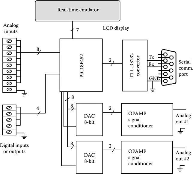
FIGURE 19.3 Schematic diagram of the hardware of the plant emulator card.

An image of the hardware realization of the plant emulator card is provided in Figure 19.4, where the physical locations of the blocks depicted in the schematic diagram of the plant emulator card are annotated with descriptive tags.

19.6 Experimental Setup of the Developed CDTRP

The experimental setup of the developed CDTRP platform is provided in Figure 19.5. It has been used for the design–test–redesigning controllers of the benchmark plants in Table 19.4 and other plants by means of operating modes given in Tables 19.1 through 19.3. The CDTRP platform setup is composed of a plant emulator card, a PC, a signal generator, power supplies, and an oscilloscope. The specifications of the plant emulator card have already been provided in Section 19.2. The PC is chosen as having a Centrino processor and a 1 GB memory, which constitute a minimum configuration necessary for running Microsoft Windows XP and MATLAB 7.04 software. The signal generator as part of the hardware peripheral unit card is included to provide external analog signal noise (D_U). Power sources constituting another part of the hardware peripheral unit card are used while DC variacs (i.e., variable power supply) are changed manually to generate the perturbations of the plant variables (D_X1, D_X2, and D_X3).

Images

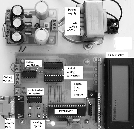
FIGURE 19.4 The hardware of the plant emulator card.

Images

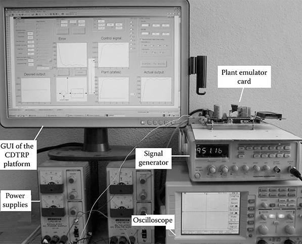
FIGURE 19.5 The experimental setup for the entire controller design–test–redesign platform.

TABLE 19.4
Benchmark Plants of Control Design—Test—Redesign Platform

Images

19.7 Verification and Validation of the Cdtrp Based on Benchmark Plants

This subsection presents experimentation results realized for verification and validation of the operating modes of the CDTRP on three physical plants and the results obtained by the investigations on reliable operating frequency of mixed modes of the CDTRP are presented in this subsection.

19.7.1 Benchmark Plants Implemented in CDTRP for Verification of Operating Modes

In this section, the benchmark plants that are implemented as simulation, emulation, or physical hardware for verification of the operating modes of the CDTRP are listed. A set of benchmark plants that can be chosen by the users via the plant selection button in the front panel of the GUI are included in the menu of the CDTRP to help the users expediently analyze their control methods on these selected benchmark plants. This menu is open to be extended by the users to cover a larger class of benchmarks or any other plants of interest. The plants must be defined by at most three-dimensional state equations.*

The benchmark plants available in the menu are listed in Table 19.4 and these are also used for verification of the operating modes of the developed CDTRP. The benchmark plants in Table 19.4 are chosen from benchmarks extensively used in the literature (which implies that they are difficult to identify and/or difficult to control) to compare the system identification methods and/or to compare the controller design methods or they are of practical importance in some other sense.

19.7.2 Controller Design, Test, and Redesign by the CDTRP on a Physical Plant: The Dc Motor Case

This section is devoted to demonstrating how to implement the controller design– test–redesign procedure introduced in the previous section to reach a controller working well for a physical plant operated under the actual environmental conditions. A micro DC motor is chosen as the plant and the final operating mode is determined as S-R-R, where the PC is used as the controller, the physical plant is the micro DC motor, the sensor, and actuator, that is, the encoder and driver are realized in a PIC microcontroller driver card (see Figure 19.6). In the initial design stage of the controller design–test–redesign procedure, the S-S-S mode was found to be the most suitable mode for one because of the simulation efficiency of the simple yet realistic DC motor models but also because of its implementation flexibility as observed in a set of experiments conducted in the S-S-S, S-E-S, and S-E-E modes.

In the test stage, the S-E-E mode was first implemented for testing the considered controller design methods on the emulated plant under emulated environmental conditions. Then, the controller candidates were analyzed in the S-E-R mode. It was found that the S-E-R mode is the most suitable mode for testing the considered control methods, since it enables analysis of the controller candidates under quite realistic conditions, while still providing flexibility in simulating different controller candidates efficiently. In the redesign stage, the S-R-S and S-R-E modes were implemented at the beginning and then the S-R-R mode was implemented as the final mode where the parameters of the controller that were found to be the best in the test stage were tuned.

* This restriction is because of the capacity limit of the chosen emulator hardware (i.e., PIC18F452).

Images

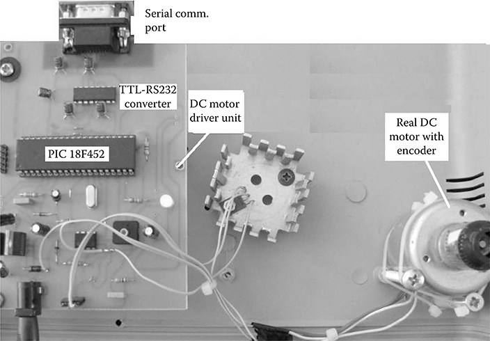
FIGURE 19.6 DC motor hardware whose driver unit is based on PIC for S-R-R mode.

The details of the above explained steps of the implementation of the controller design–test–redesign procedure for the DC motor example are presented next.

19.7.2.1 Implementation of the Physical Plant Together with Its Physical Actuator and Sensor Units

A micro DC motor was considered. The DC motor driver card (see Figure 19.6) was realized with a PIC18F452 microcontroller driver unit that has a serial interface to communicate with the PC. The speed of the motor was considered as the output and was measured by an encoder to provide feedback to the system. The microcontroller-based driver unit drives the DC motor speed revolutions per minute (rpm) via pulse width modulation (PWM) changing between 0% and 100%. That is to say, in the implemented S-R-S, S-R-E, and S-R-R operating modes, the control signal from CDTRP is converted into a PWM signal to control physical DC motor speed rpm.

19.7.2.2 Identification of DC Motor to Obtain a Model to be Simulated and Emulated

To simulate and also emulate the physical DC motor in the simulated-plant and emulated-plant modes that are to be used for the design and test stages, a system identification procedure was applied to the physical DC motor and then the simplest yet realistic model for the considered micro DC motor was obtained.*

A step function, which is obtained by changing PWM sharply, was fed to the physical DC motor plant. The input–output data pairs of the plant necessary for the identification were measured via the hyper-terminal of the PC. After the process of data gathering, the transfer function of the plant was found under the assumption of a single-input single-output linear dynamic system for the plant. It is known [44,51] that the physical DC motor plant can be well modeled as a first-order delayed dynamic system according to the response of the plant due to the step input. The step response of the first-order system defined with three parameters is provided in the Laplace and time domain, respectively, as follows:

H (s) = \frac{K}{T s + 1} e^{- L s} (19.1)

$H (s) = \frac{K}{T s + 1} e^{- L s} (19.1)$

h (t) = K (1 - e^{- (t - L) / T}) ≅ K (1 - e^{- t / T}) (19.2)

$h (t) = K (1 - e^{- (t - L) / T}) ≅ K (1 - e^{- t / T}) (19.2)$

where T is the time constant, L is the dead-time, and K is the gain [52]. If the dead-time L is sufficiently small compared to the time constant T of the plant, the step response of the system can be approximated as shown in Equation 19.2. Thus, a first-order micro DC motor model (BP5 in Table 19.4) was obtained with the measured maximum motor speed 4224 rpm, the time constant 0.5 s, and the dead-time 0.011 s. This model was used for the S-S-S, S-E-S, S-E-E, S-E-E, and S-E-R operating modes of the CDRTP. Although the first-order system is sufficient to model the physical micro DC motor for testing the candidate controllers, a second-order model is also identified and implemented for validating the emulator of the platform by analyzing the emulation performance of the platform with a more realistic model. The considered second-order delay dynamic system model is defined in the Laplace domain as follows:

H (s) = \frac{K w_{n}^{2}}{s^{2} + 2 ζ w_{n} s + w_{n}^{2}} e^{- L s} (19.3)

$H (s) = \frac{K w_{n}^{2}}{s^{2} + 2 ζ w_{n} s + w_{n}^{2}} e^{- L s} (19.3)$

P_{o} = e^{- \frac{ζ π}{\sqrt{1 - ζ^{2}}}} (19.4)

$P_{o} = e^{- \frac{ζ π}{\sqrt{1 - ζ^{2}}}} (19.4)$

T_{s} = 3 τ = \frac{3}{ζ w_{n}} (19.5)

$T_{s} = 3 τ = \frac{3}{ζ w_{n}} (19.5)$

* It should be noted that although more complicated models better suited to the real data measured from the DC motor can be derived, it was preferred to work with this simple model for the plant. Not only does the simple model allow taking advantage of efficient simulation and emulation of the DC motor, but it also allows more focus on testing the controllers’ performances on the considered DC motor and on its simulated/emulated model in a comparative way, rather than on simulating/emulating the DC motor more realistically by more complicated models. In fact, it was observed that choosing a simple first-order dynamic model for the DC motor that was identified by using a step response method provides sufficiently close responses to the ones measured from the physical DC motor and also enables seeing the differences among the performances of the different controllers implemented.

where K is the gain, L is the dead-time, ζ is the damping ratio, and w_n is the natural frequency. The damping ratio and natural frequency were determined from the P_o overshoot percentage in Equation 19.4 and T_s settling time in Equation 19.5 [52]. The second-order micro DC motor model was obtained based on the measured P_o of 10%, T_s of 4.46, and the dead-time of 0.011 s.

19.7.2.3 Recreating The Disturbance And Parameter Perturbation Effects

The disturbance and parameter perturbation effects that can be implemented in the emulator by means of the signal generator and power supply components of the hardware peripheral unit were produced in the implemented S-E-R and S-R-R modes to recreate an actual environment. Since there is no such interface possibility of the simulators running on the PCs and emulators in the simulation/emulation platforms known in the literature, this is a unique feature of the developed CDTRP platform.

19.7.2.4 Controller Design–Test–Redesign Process

The DC motor speed tracking problem was chosen as a case study. The following four different types of controllers were designed using mainly the S-S-S, S-E-S, and S-E-E modes, then tested using the S-E-E and S-E-R modes on the identified model BP5, and finally using the S-R-S, S-R-E, and S-R-R modes on the realized micro DC motor: (1) a proportional-integral-derivative (PID) controller designed by the Ziegler–Nichols (ZN) method [13,14,52], (2) a PID controller designed by the Chien, Hrones, and Reswick (CHR) method [53], (3) a robust controller designed by the partitioned robust control (PRC) method [54], and (4) a direct adaptive controller designed by the Model Reference Adaptive Control (MRAC) method [54].

A PID controller that defines the control signal u in terms of the error is given as follows:

u = K_{p} e + K_{i} \int e d t + K_{d} \dot{e} (19.6)

$u = K_{p} e + K_{i} \int e d t + K_{d} \dot{e} (19.6)$

where e is the error between the desired and actual output of the plant, ė is the derivative with respect to time of the error, and K_p, K_i, and K_d are the proportional, integral, and derivative gain parameters, respectively. In the first method, the parameters of the PID controller were calculated based on the BP5 plant model as K_p = 54.54, K_i = 2479.3, and K_d = 0.3 by using the ZN step response method. In the second method (CHR), which was preferred for yielding minimum overshooting [12], the PID controller parameters were calculated * as K_p= 43.18, K_i = 1635.6, and K_d = 0.1995. The PRC is designed as having two separate parts: (1) proportional-derivative (PD) control u_e and (2) auxiliary control u_y [54,55]. In this method, given a plant model ẋ = −ax + bu (e.g., BP5 model), the control signal was calculated as follows:

u = u_{e} + u_{y} = K_{v} \dot{e} + K_{p} e - a x - Δ a x (19.7)

$u = u_{e} + u_{y} = K_{v} \dot{e} + K_{p} e - a x - Δ a x (19.7)$

where K_v and K_p gains related to the control input u_e were chosen greater than zero, and for the auxiliary controller u_y∆a = 1.2a was chosen for removing the parameter perturbations and plant uncertainties. In the fourth method applied, the MRAC controller is composed of a first-order reference modelẋ_m, two adaptive controller parameters ${\dot{u}}_{y}^{k}$ ${\dot{u}}_{y}^{k}$ , ${\dot{u}}_{r}^{k}$ ${\dot{u}}_{r}^{k}$ , and a control signal u as follows:

* The considered PID controller is actually redesigned at this step within the terminology introduced in this chapter.

\begin{array}{l} {\dot{x}}_{m} = - a_{m} x_{m} + b_{m} r \\ {\dot{u}}_{y} = - λ (x_{m} - x) y a_{m} (e^{- a_{m}}) \\ {\dot{u}}_{r} = - λ (x_{m} - x) r a_{m} (e^{- a_{m}}) \\ u = u_{r} + u_{y} \end{array} (19.8)

$\begin{array}{l} {\dot{x}}_{m} = - a_{m} x_{m} + b_{m} r \\ {\dot{u}}_{y} = - λ (x_{m} - x) y a_{m} (e^{- a_{m}}) \\ {\dot{u}}_{r} = - λ (x_{m} - x) r a_{m} (e^{- a_{m}}) \\ u = u_{r} + u_{y} \end{array} (19.8)$

where y stands for the actual output, r stands for the reference signal, the designed parameter was chosen as λ = 0.5, and the values of the reference model parameters a_m and b_m are two times the values of the BP5 plant parameters. The equations in Equation 19.8 generate the control signal.

19.7.2.5 The Simulation, Emulation, and Physical Measurement Results Obtained along the Entire Design Process Implemented by CDTRP

The step responses of the physical DC motor and the BP5 implemented in the emulator (both controlled by the same controllers designed with the above-mentioned methods) for the desired output of 2500 rpm are given in Figure 19.7a through d, respectively. It can be seen from the responses depicted in Figure 19.7 that one may prefer the first two controllers, that is, the ones designed by the ZN and CHR methods, since the step responses of the emulator have relatively short rise times and are close to the reference signal, that is, the step function. However, the responses of the physical DC motor controlled by these two controllers for the same step input are not close to the emulated first-order model responses in the sense that the physical DC motor demonstrates second-order dynamic behavior rather than first-order.* On the contrary, the responses to the step input of the physical DC motor and the emulated first-order model are very close to each other for the MRAC case.

Images

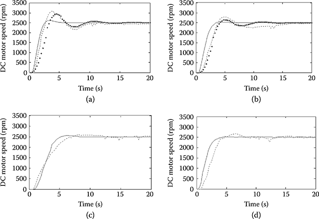
FIGURE 19.7 Physical DC motor S-R-R results (dashed), real-time emulator S-E-S results for first-order model (solid), and real-time emulator S-E-S results for second-order model (dotted) with (a) a proportional-integral-derivative (PID) controller whose parameters are designed by the Ziegler–Nichols method, (b) a PID controller whose parameters are designed by the Chien, Hrones, and Reswick method, (c) a partitioned robust controller, and (d) a Model Reference Adaptive controller.

The following can then be concluded: (1) it can be expected that the real plant will behave similar to the emulator for the PRC and MRAC even if the plant model poorly reflects the behavior of the physical plant and (2) it can be expected that the physical plant will behave similar to the emulator for the PID controllers designed by the ZN and CHR methods only when the plant model is realistic so as to be capable of reflecting the behavior of the real plant well. So, the analysis results obtained from the developed CDTRP in the emulated-plant and also the simulated-plant modes are reliable on the realistic plant models for any kind of controller design methods and further reliable even on poor plant models for the PRC and MRAC design methods.

19.7.2.6 Recreating the Parameter Perturbations in the S-E-R Mode

Parameter perturbations were created as a multiplicative effect for the model parameters. The perturbation signals were provided by DC power source in the 0–5 V (DC) range and were fed to the hardware peripheral unit card via the D_X1 port that was activated by the ADC options in the GUI, where 1 V for D_X1 corresponds to the nominal plant parameters case. The observed responses of the emulated BP5 controlled by the PRC for four different parameter values are given in Figure 19.8a. The responses observed for the MRAC case are given in Figure 19.8b. In addition, the responses obtained for the PRC and MRAC are compared to each other in terms of their performances for two parameter perturbation values in Figure 19.9. No results are depicted for the PID controller case, since it behaves very poorly in the face of parameter variations. It can be said that the responses under parameter variations are close to each other for the PRC and MRAC. As observed in the above analysis part, (1) choosing more realistic models yields better emulation results to be obtained by the CDTRP platform and (2) for the MRAC and to a lesser extent for the PRC cases, the responses of the emulator are very close to the physical plant. In light of these facts, it may be concluded that the performances of the controllers on the physical plants under parameter perturbations can be examined using S-E-R mode in the manner that the CDTRP implements.

19.7.2.7 Recreating Noise Disturbance in the S-E-R Mode

Noise disturbances were created as additive to the control signal (i.e., input of the plant model). The noise signal was provided by the signal generator whose range is given in Table 19.5. It was fed to the hardware peripheral unit card via D_U port that is activated by the ADC options in the GUI. The noise signal amplitude can be scaled via the front panel of the GUI for CDTRP applications. For the noise signal du = 0.1 sin(2πf) with f = 1Hz, which was created by the noise scaling factor of 0.1 set by using the front panel of the GUI, the corresponding responses obtained for PID, PRC, and MRAC are given in Figure 19.10. As expected, the CDTRP confirms that the PID has quite poor performance under the applied additive noise, whereas the PRC and MRAC perform well. It should be noted that the MRAC shows the best steady state performance.

* As seen in Figures 19.7a and b, the responses of the emulated second-order system model are much closer to the real DC motor responses.

Images

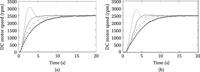
FIGURE 19.8 Responses of BP5 to the step input for parameter variation coefficients of 0.5 (dashed, --), 1 (solid, -), 1.5 (dotted-solid, -·), and 2 (dotted on solid, -·-). Note that the coefficient values are the factors multiplying the nominal parameter value to obtain the perturbed parameter. The responses in (a) and (b) are for the partitioned robust controller and the Model Reference Adaptive controller, respectively.

Images

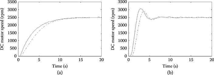
FIGURE 19.9 Responses of BP5 to the step input for the parameter variation coefficients of 2 in (a) and 0.5 in (b). The responses (solid) and (dotted-solid, -·) were obtained for the partitioned robust controller and the Model Reference Adaptive controller, respectively.

TABLE 19.5
Noise Disturbances Range Scaling

Volt (Ac) From Signal Generator	Volt (Dc) for Adc
+1 V	5 V
0 V	2.5 V
–1 V	0 V

Images

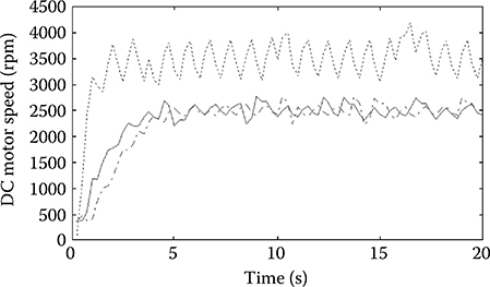
FIGURE 19.10 Responses of the emulator controlled by proportional-integral-derivative controller (dashed, --), partitioned robust controller (solid, -), and Model Reference Adaptive controller (dotted-solid, -·) under the noise du = 0.1 sin(2π1t).

19.7.2.8 Response to Single Short-in-Time Large-in-Amplitude Pulse Disturbance in the S-E-R and S-R-R Modes

Recreating the effects of relatively small amplitude noise disturbances in the emulation have been presented above. Now, another kind of disturbance effect, that is, a single short-in-time and large-in-amplitude pulse disturbance effect was created and applied to both the emulated BP5 model and the physical DC motor. This enables a better understanding of the validity of the developed platform in mimicking the behavior of the physical plants under actual disturbances. The disturbance was created as a multiplicative effect to the output of the model. The pulse time and amplitude were chosen in the front panel of the GUI. In the tests, the pulses were created after the transient regime (e.g., at 10 s as shown in Figure 19.11) to mimic the disturbances appearing in the steady state working conditions for the plant. The measured responses of the physical DC motor and the emulator controlled by the PID, robust, and MRAC controllers are given in Figure 19.11.

19.7.3 Investigation of Reliable Operating Frequency of Mixed Modes of CDTRP: Coupled Oscillators as Benchmarks

All mixed operating modes of CDTRP require at least two of the controller, plant, and peripheral components to be implemented in different units of CDTRP, that is, in two of the simulator (PC), the emulator, and the hardware peripheral unit. So, the mixed modes necessitate real-time compatibility of the PC, emulator, and hardware peripheral unit. In other words, these units have to communicate in a (real-time) synchronized fashion. To examine this ability of the CDTRP, Lorenz systems–based chaotic synchronization is chosen as the benchmark application. As will be seen below, chaotic synchronization is a good example to understand the operating (frequency) limits of the CDTRP.

Images

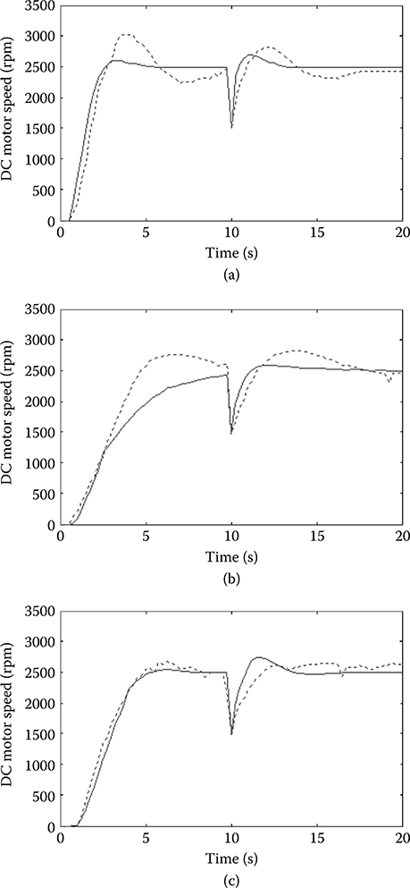
FIGURE 19.11 Responses of the physical DC motor and the emulator controlled by the proportional-integral-derivative (whose parameters are calculated with the Ziegler-Nichols method), robust, and Model Reference Adaptive controllers are given, respectively, in (a), (b), and (c). The pulse amplitude is chosen as k = 0.6 and the time when the pulse is applied as 10 s. Note that (dashed, --) is for the physical plant and (solid, -) is for the emulator of CDTRP.

The following were observed * in a set of experiments conducted:

The emulator and the simulator cannot be synchronized to each other and to external hardware because of the high frequency dynamics intrinsic to the chaotic (Lorenz) system.
As a consequence of the maximum achievable sampling frequency that can be realized in the MATLAB environment used for the PC simulator and in the emulator implemented by using the PIC microcontroller, the simulator and the emulator of the developed CDTRP can be synchronized to each other when implementing the dynamics up to 25 Hz while the simulator and the emulator can implement the dynamics up to 300 Hz and 25 Hz, respectively, if they are operated as uncoupled.
The frequency range of the simulated/emulated system dynamics for which mutual synchronization among the emulator, the simulator, and the external hardware are achievable can be enlarged by using a suitable feedback control.

In the sequel, the experimental results obtained for a set of different kinds of implementations of synchronized coupled Lorenz systems are given first and then the coupled linear undamped pendulums are examined to find the limit for the frequency that enables synchronous operation for the implemented dynamics.

19.7.3.1 Analog Hardware Implementation of Synchronized Lorenz Chaotic Systems

Before examining the CDTRP in the E-R-R and R-E-R operating modes for the synchronized system of coupled Lorenz systems, the systems were first implemented as analog hardware (i.e., in the R-R-R mode). The master–slave configuration proposed in Cuomo et al. [56] was used for the implementation. The transmitter and receiver circuits of the Lorenz chaotic systems, whose scaled state equations are given as BP9 and BP10, respectively, in Table 19.4, were realized with the circuit configuration in Figure 19.12 using the analog multiplier AD633, opamp LF353, and passive circuit elements (R1 = R2 = R6 = R7 = 100 kΩ, R3 = R5 = R8 = R10 = 10 kΩ, R4 = R9 = 1 MΩ, RV1 = RV3 = 100 kΩ, RV2 = RV4 = 220 kΩ, and C1 = … = C6 = 100 nF).^† The synchronization result for the analog hardware realization of the master–slave synchronization of the coupled systems is shown in Figure 19.13.

19.7.3.2 Synchronization of (Lorenz Ttransmitter) Emulator with a Physical Analog (Lorenz Receiver) Plant

As a second implementation of master–slave synchronization of coupled Lorenz systems, the CDTRP was operated in the E-R-R mode such that the transmitter BP9 was implemented in the emulator of the CDTRP and the receiver implemented as analog hardware shown in Figure 19.12 was used as the plant. The X1 state was observed from the hardware peripheral unit card via the DAC port that was activated by the DAC options in the GUI. The implementation of the system in E-R-R mode is given in Figure 19.14. As seen in Figure 19.15, when operating in the E-R-R mode, the emulator of the CDTRP can roughly mimic the chaotic behavior of the Lorenz system. In this E-R-R mode, the master Lorenz system was realized in the emulator and the slave Lorenz system was realized in the analog hardware. During the experiments, such master–slave coupled Lorenz systems were never observed as synchronized.

* It should be noted that the last (interesting) observation can be interpreted as follows: The interfaces among the simulator, emulator, and external hardware have delays due to the interrupt routines, which can be modeled by (complex frequency) poles determining an upper cutoff frequency. And, where the synchronization is achieved, these poles that limit the frequency range can be shifted to a higher frequency point by using feedback control.

† Note that the circuit configuration was chosen as given in Paul [57] but with the BP9-BP10 coefficients as β = 10, r = 56.6, and b = 5.02. For the coefficients, the Lorenz systems then produce chaotic oscillations with the main harmonics around 8.5 Hz.

Images

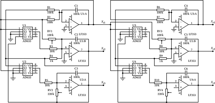
FIGURE 19.12 Realized analog circuit for master–slave synchronization of Lorenz chaotic systems.

Images

FIGURE 19.13 A snapshot in the X-Y mode of the oscilloscope where the signals in the X and Y channels are the first state variables of the master and slave Lorenz circuits, respectively.

Images

FIGURE 19.14 Implementation of the E-R-R mode of the controller design–test–redesign platform for the synchronized Lorenz systems.

Images

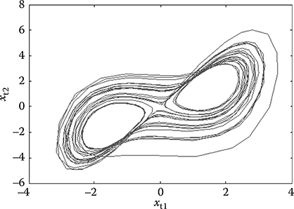
FIGURE 19.15 Phase portrait for the x_t1 and x_t2 states of the emulated BP9 Lorenz chaotic system as observed via the graphical user interface when the controller design–test–redesign platform is operated in the E-R-R mode.

19.7.3.3 Synchronization of the (Lorenz Receiver) Emulator with Physical Analog (Lorenz Transmitter) Hardware

As a third implementation of master–slave synchronization of coupled Lorenz systems, the CDTRP was operated in the R-E-R mode such that the receiver BP10 was implemented in the emulator of the CDTRP and the transmitter implemented as analog hardware shown in Figure 19.12 was used as the master. The X1 state was applied to the emulator of the CDTRP via the hardware peripheral unit card by the X1 port that was activated by the ADC options in the GUI. The implementation of the R-E-R mode is given in Figure 19.16.

As seen in Figure 19.17, when operating in the R-E-R mode, the emulator of the CDTRP fails to mimic the chaotic behavior of the Lorenz system. In this R-E-R mode of operation, the master Lorenz system was implemented in the analog hardware card and the slave Lorenz system was implemented in the emulator. During the experiments conducted for this realization of the master–slave Lorenz system, synchronization was never observed.

Images

FIGURE 19.16 Implementation of the R-E-R mode of the controller design–test–redesign platform for the synchronized Lorenz systems.

Images

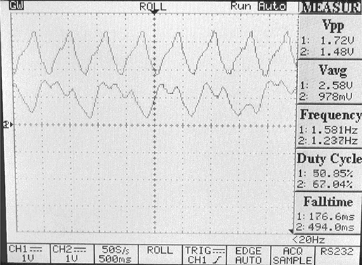
FIGURE 19.17 First state variables of the analog transmitter and the emulated receiver in the R-E-R mode for synchronized Lorenz systems. The receiver state is the top trace and the transmitter state is the bottom trace.

19.7.3.4 Synchronization of (Lorenz Transmitter) Simulator with (Lorenz Receiver) Eemulator

As a fourth implementation of master–slave synchronization of coupled Lorenz systems, the CDTRP was operated in the S-E-E mode such that the receiver BP10 was implemented in the emulator of the CDTRP and the transmitter was implemented in the simulator of the CDTRP. As seen in Figure 19.18, although both the simulator and emulator can roughly mimic the chaotic behavior of the Lorenz system, they fail to be synchronized to each other in the master–slave configuration.

19.7.3.5 Effect of Feedback on Chaotic Synchronization

The above implemented master–slave configuration for chaotic synchronization is, indeed, an open loop control system where the receiver is the plant and the transmitter output is the reference signal to be tracked by this plant. One can argue that not only the lack of implementing the high frequency components of the chaotic signals is the source of failure to achieve the chaotic synchronization, but also the master–slave configuration is another source of dissynchronization as this open loop control configuration is sensitive to internal/external disturbances and delays. To clarify this point, in a unity feedback closed loop configuration, a PID controller with the parameters K_p = 1, K_i = 100, and K_d = 0.01 is used to provide a suitable control input to the receiver Lorenz system for deriving its output to track the reference chaotic signal produced by the transmitter Lorenz system. As seen in Figure 19.19, the PID controller with unity feedback closed-loop configuration provides the desired synchronization for the Lorenz receiver system whose output tracks the reference chaotic signal at least for the main harmonics corresponding to low frequency components.

Images

FIGURE 19.18 Time waveforms of the first states of the Lorenz transmitter and receiver, which are implemented in the simulator and the emulator, respectively.

Images

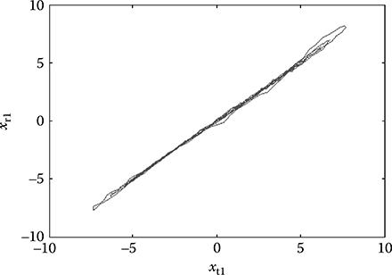
FIGURE 19.19 First state variable of the receiver Lorenz system as compared to the reference signal, which is the first state variable of the transmitter Lorenz system in the S-E-E mode.

The above-mentioned limits of the CDTRP in implementing the synchronized Lorenz systems are natural consequences of the chaotic dynamics of the Lorenz systems that intrinsically possess high frequency components. Moreover, the implementation is limited by the maximum achievable sampling frequencies that can be realized in the MATLAB environment used for the PC simulator and in the emulator implemented by the PIC microcontroller. As seen in the last closed-loop implementation of coupled Lorenz systems based on a simple PID controller, the synchronization can be achieved by using a suitable feedback at least for the main (low frequency) harmonics of the chaotic signals. The exact frequency range for the control system dynamics that allows synchronous operations of the units of the CDTRP platform in implementing these dynamics was investigated by considering what may be the simplest yet challenging example, namely the linear undamped pendulums. The corresponding results are presented in the next section.

19.7.3.6 Synchronization of (Linear Undamped Pendulum Receiver) Simulator/Emulator with (Signal Generator Transmitter) Simulator

To determine the reliable operating frequency range for the simulator and emulator when communicating with each other, first, a signal generator was used as a transmitter in a master–slave configuration for deriving the emulator or simulator where the BP8 pendulum model was implemented (Figure 19.20a). Then, a PID controller with parameters K_p = 1, K_i = 100, and K_d = 0.001 in the unity feedback closed-loop configuration was used to control the receiver pendulum to track the output of the signal generator. For both the configurations, the CDTRP was operated in the S-E-E mode and also in the S-S-S mode (Figure 19.20b.). It was observed that both the implemented modes yield almost identical results up to f =25 Hz, as shown by the results obtained for the S-S-S mode given in Figure 19.21.

Images

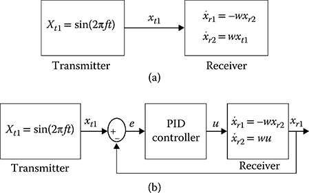
FIGURE 19.20 (a) Receiver emulator or simulator was derived by a simulated signal generator (x_t1) in open-loop master–slave configuration for S-S-S or S-E-E modes of the controller design–test–redesign platform. (b) Receiver emulator or simulator was derived by a simulated signal generator (x_t1) in closed-loop for S-S-S or S-E-E modes of the controller design–test–redesign platform.

On the one hand, in the open-loop configuration, the synchronization that was achieved for f = 1 Hz was observed to fail beyond f = 10 Hz. On the other hand, in the closed-loop configuration, it was observed that the synchronizations sustained up to f = 100 Hz and f = 25 Hz in the S-S-S mode and the S-E-E mode, respectively. These observations actually determine the limit of the operating frequency for the control systems dynamics whose real-time implementations in the S-E-E and S-S-S modes of the CDTRP are reliable in the sense that they can be considered as valid real-time implementations.

19.7.3.7 Synchronization of (Linear Undamped Pendulum) Receiver Emulator with (Signal Generator) Transmitter

To determine the reliable frequency range for the emulator in the R-E-E and R-E-R modes of CDTRP where it receives a signal from external analog hardware, the receiver BP8 was implemented in the emulator and analog signal generator test equipment was used for the transmitter as shown in Figure 19.22. The x_t analog signal was applied to the emulator via the hardware peripheral unit card by the U port that was activated by the ADC options in the GUI. The difference between the experiments done in the S-E-E mode shown in Figure 19.20 and in the R-E-E and R-E-R modes shown in Figure 19.22 is in the transmitter part such that in the former one the transmitter is realized in the simulator and in the other ones the transmitter is realized in analog hardware. The analog signal received by the emulator and also the output of the pendulum created in the emulator are transferred from the emulator to the GUI. Therefore, the unique additional source of limiting the frequency range of the emulated dynamics in this experiment is the usage of the input U port of the emulator operated by the ADC. As shown in Figure 19.23, it was observed that in the open-loop configuration of Figure 19.22, the synchronization was achieved up to f = 1.52 Hz. It should be noted that the relatively narrower frequency range than the one obtained for S-E-E mode was due to the ADC interface of the PIC microcontroller.

Images

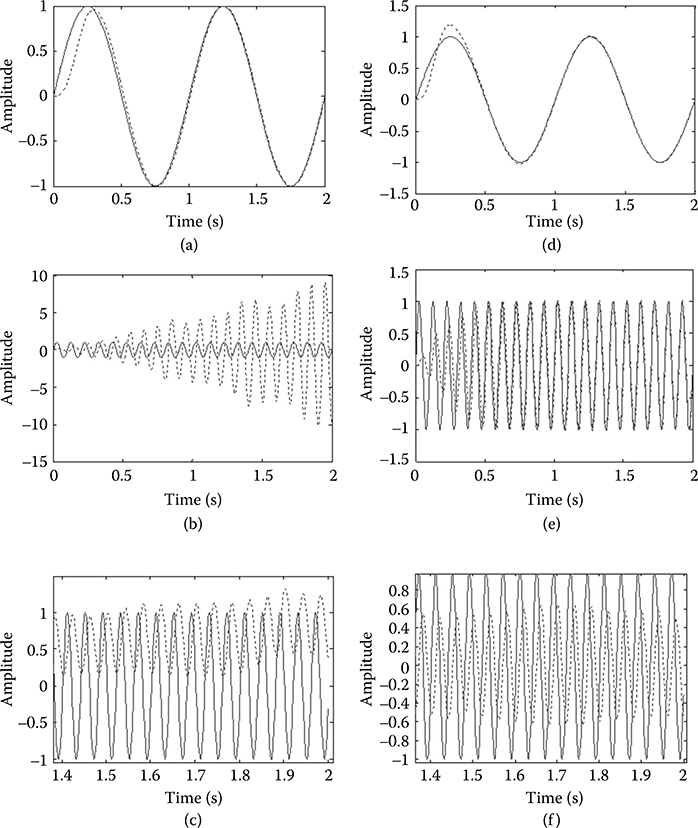
FIGURE 19.21 (a) Master–slave synchronization at f = 1 Hz. (b) Master–slave synchronization failure at f = 10 Hz. (c) Master–slave synchronization failure at f = 100 Hz. (d) Proportional-integral-derivative (PID)-based closed-loop synchronization at f = 1 Hz. (e) PID-based closed-loop synchronization at f = 10 Hz. (f) PID-based closed-loop synchronization at f = 100 Hz. Note that (dashed, --) is for the receiver (pendulum) signal and (solid, -) for the transmitter (generator) signal in S-S-S mode of the controller design–test–redesign platform.

Figure 19.22b shows that the above given frequency limit can be extended up to f = 2.92 Hz (Figure 19.24) by using a PID controller with the parameters K_p = 1, K_i = 100, and K_d = 0.001 in the unity feedback closed-loop configuration for controlling the receiver pendulum to track the output of the analog signal generator. The PID controller was implemented as analog hardware (Leybold LH 734 06 PID-Controller Lab Equipment), so the CDTRP was operated in the (closed-loop) R-E-E and R-E-R modes. Note that the frequency limit is lower than f = 25 Hz, which is the one observed for the closed-loop (signal generator–pendulum) synchronization in the S-E-E mode since the analog output of the DAC interface of the plant emulator card was also used in addition to the analog input of the ADC interface of the emulator.* The above results show that the real-time implementations of the control systems dynamics realized in the R-E-E and R-E-R modes are reliable up to the f = 2.92 Hz frequency.

Images

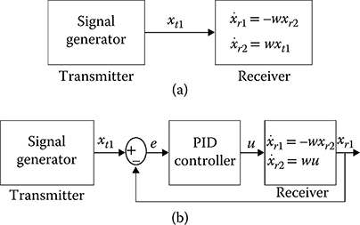
FIGURE 19.22 (a) Receiver (pendulum) emulator was derived by analog signal generator (b) Receiver (pendulum) emulator controlled by a proportional-integral-derivative controller tracks transmitter signal in R-E-E and R-E-R modes.

Images

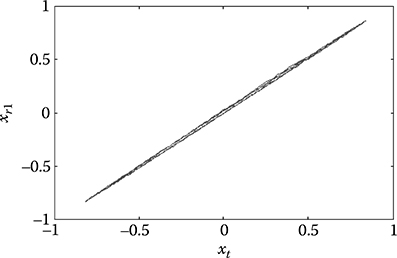
FIGURE 19.23 Master–slave synchronization between analog generator signal and first state of pendulum realized in the emulator as observed from data transferred to graphical user interface.

Images

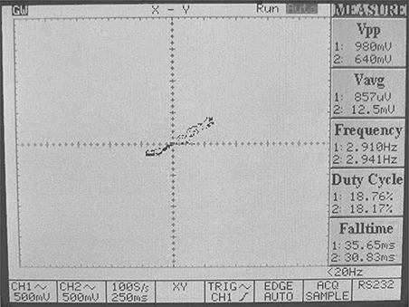
FIGURE 19.24 A snapshot on the X-Y mode of the oscilloscope where the signals in the X and Y channels are the signal generator signal and the pendulum emulator output, respectively, in the R-E-E and R-E-R modes.

19.7.3.8 Synchronization of a Physical Analog (Lorenz Receiver) Hardware with Transmitter Emulator

As the last implementation, the emulator implementing transmitter was used for deriving an analog receiver, that is, the Lorenz system. Then, the reliable frequency range for the emulator in the E-R-E and E-R-R modes of CDTRP was examined. The pure sinusoidal signal generated in the emulator was applied via the DAC interface of the emulator in an additive manner to the first state of the Lorenz system implemented in the hardware peripheral unit card (see Figure 19.25). Note that the Lorenz system was realized by the capacitances for reducing the main harmonics of the chaotic signal around the maximum reliable real-time operation frequency of the emulator. The source of limiting the frequency range of the implemented dynamics in this experiment is the usage of analog output of the DAC interface of the plant emulator card. As shown in Figures 19.26 and 19.28, it was observed that the synchronization is achieved up to f = 4.05 Hz in the open-loop configuration of Figure 19.28 and achieved up to f = 9.09 Hz for the closed-loop configuration with a PID controller with the parameters K_p = 1, K_i = 100, and K_d = 0.001 in the unity feedback in Figure 19.27 (where Leybold LH 734 06 PID-Controller Lab Equipment was used again).

It should be noted that the Lorenz system derived by the pure sinusoidal transmitter signal did not exhibit a chaotic Lorenz signal for the large amplitude values of transmitter signal anymore and that the synchronization was indeed achieved for the main harmonic of the disturbed Lorenz signal. So the phase synchronizations seen in Figures 19.26 and 19.27 were not exact because of the subharmonics. The subharmonics appear as a consequence of the considered operating mode, which requires the implementation of a part of the Lorenz system in the analog hardware and the other part in the emulator so that their interface is a source of nonlinearity causing subharmonics. The results show that the real-time implementations of the control systems dynamics realized in the E-R-E and E-R-R modes are reliable up to the f = 9.09 Hz frequency.

* Observe from Figure 19.22 that the analog output of the emulator was fed to the oscilloscope and also to the analog PID hardware.

Images

FIGURE 19.25 Transmitter emulator derives analog Lorenz system receiver in E-R-E and E-R-R modes of the controller design–test–redesign platform (a chaotic state modulation system where a transmitter signal is injected into the chaotic system as additive to the first state).

Images

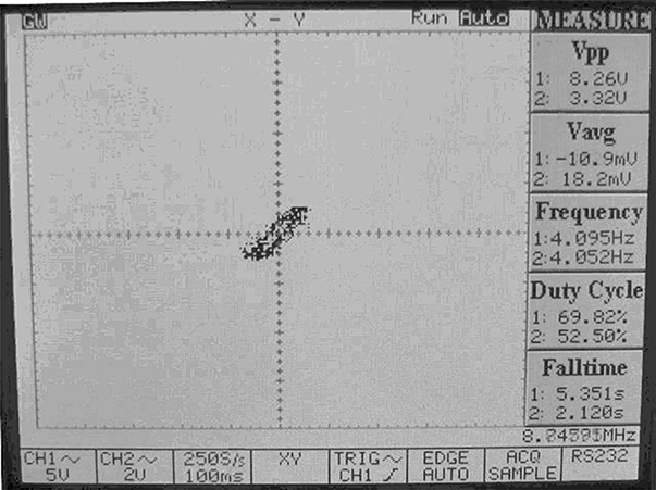
FIGURE 19.26 A snapshot on the X-Y mode of the oscilloscope where the signals in the X and Y channels are the transmitter signal and the first-state variable of the Lorenz system, respectively.

Images

FIGURE 19.27 A snapshot in the X-Y mode of the oscilloscope where the signals in the X and Y channels are the transmitter signal and the first-state variable of the Lorenz system, respectively, in proportional-integral-derivative-based closed-loop control.

Images

FIGURE 19.28 Proportional-integral-derivative-based closed-loop control for Lorenz system receiver to track output of the transmitter emulator in E-R-E and E-R-R modes of the controller design–test–redesign platform.

19.8 Conclusions

A real-time simulation platform called CDTRP has been developed, verified, and validated. The developed platform consists of a simulator together with a software manager in PC (i.e., GUI), microcontroller-based emulator, and hardware peripheral unit. This platform is devoted to controller design, test, and redesign with an emphasis on recreating actual operating conditions for examining and analyzing the actual performance of designed controllers while still having the opportunity to modify and tune the controller candidates based on their performances in a flexible way and without causing any damage to the physical plant or creating dangerous situations. CDTRP enables the embedding, via its hardware peripheral unit, of actual disturbances and any part or accessories of a physical plant. For example, actuators and sensors can be implemented in laboratory conditions while the other parts of a plant are implemented in the simulator or emulator of the platform. This configurability enables users to approximate the physical plants and their actual environments as closely as desired. So, the developed CDTRP can be used for the design–test– redesign of controllers, comparison of the performances of the different controller algorithms, and controller parameter training procedures.

The real-time simulation modes (e.g., “hardware-in-the-loop simulation,” “control prototyping,” and “software-in-the-loop simulation”) are realized with the developed CDTRP because it can be operated in 24 different real-time operating modes where the controller, plant, and peripheral unit are implemented either in the simulator, in the emulator, or realized by external analog or digital hardware depending on the application and requirements on, for example, memory and time complexity. A subset of the operating modes that are introduced in this chapter contribute to the real-time simulation literature while the remaining ones correspond to the well-known simulation modes in the literature. The operating modes are described in a novel taxonomy and categorized based on their suitability to the design, test, and redesign stages of the proposed controller design process.

As observed by the investigation conducted in this work, the capabilities of the CDTRP platform in implementing the controllers and plants are limited by the hardware and software realizations used for its simulator and emulator units. This includes the MATLAB environment used for the PC simulator, a PIC microcontroller to implement the emulator, and the communication between these two and the external hardware units. The frequency range for a reliable implementation of the operating modes of the CDTRP was determined by measuring the phase synchronization between the coupled oscillators, which are realized in different units of CDTRP.

The proposed design, test, and redesign procedure can be used in any simulation platform that provides a hierarchy of operating modes ranging from the flexible ones to the ones close to physics, and the developed platform is open to be improved in some focused control applications.

References

1. Doyle, J. C., B. A. Francis, and A. R. Tannenbaum. 1992. Feedback Control Theory. New York: Macmillan.

2. Goodwin, G. C., S. F. Graebe, and M. E. Salgado. 2001. Control System Design. Engelwood Cliffs, NJ: Prentice-Hall.

3. Mandal, A. K. 2006. Introduction to Control Engineering Modeling, Analysis and Design. New Delhi, India: New Age International Limited Publishers.

4. Keel, L., J. Rego, and S. Bhattacharyya. 2003. “A New Approach to Digital PID Controller Design.” IEEE Transactions on Automatic Control 48 (4): 687–92.

5. Yamamoto, T., K. Takao, and T. Yamada. 2009. “Design of a Data-Driven PID Controller.” IEEE Transactions on Control Systems Technology 17 (1): 29–39.

6. Mehta, S. and J. Chiasson. 1998. “Nonlinear Control of a Series DC Motor: Theory and Experiment.” IEEE Transactions on Industrial Electronics 45 (1): 134–41.

7. Pellegrinetti, G. and J. Bentsman. 1996. “Nonlinear Control Oriented Boiler Modeling—A Benchmark Problem for Controller Design.” IEEE Transactions on Control Systems Technology 4 (1): 57–63.

8. Güvenç, B. A. and L. Güvenç. 2002. “Robust Two Degree-of-Freedom Add-on Controller Design for Automatic Steering.” IEEE Transactions on Control Systems Technology 10: 137–48.

9. Lin, F. J. 1997. “Real-Time IP Position Controller Design with Torque Feedforward Control for PM Synchronous Motor.” IEEE Transactions on Industrial Electronics 44: 398–407.

10. Rodriguez, F. and A. Emadi. 2007. “A Novel Digital Control Technique for Brushless DC Motor Drives.” IEEE Transactions on Industrial Electronics 54 (5): 2365–73.

11. Betin, F., A. Sivert, A. Yazidi, and G.-A. Capolino. 2007. “Determination of Scaling Factors for Fuzzy Logic Control Using the Sliding-Mode Approach: Application to Control of a DC Machine Drive.” IEEE Transactions on Industrial Electronics 54: 296.

12. Boyd, S. P. and C. H. Barratt. 1991. Linear Controller Design: Limits of Performance. Englewood Cliffs, NJ: Prentice-Hall.

13. Ziegler, J. G. and N. B. Nichols. 1942. “Optimum Setting for Automatic Controllers.” ASME Transactions 64: 759–68.

14. Ogata, K. 1997. Modern Control Engineering. 3rd ed. Englewood Cliffs, NJ: Prentice-Hall.

15. Bishop, R. H. 2008. The Mechatronics Handbook. 2nd ed. Boca Raton, FL: CRC Press.

16. Zeigler, B. P. and J. Kim. 1993. “Extending the DEVS-Scheme Knowledge-Based Simulation Environment for Real-Time Event-Based Control.” IEEE Transactions on Robotics and Automation 9 (3): 351–6.

17. Maclay, D. 1997. “Simulation Gets into the Loop.” Institute of Electrical and Electronics Engineers 43 (3): 109–12.

18. Bacic, M. 2005. “On Hardware-in-the-Loop Simulation.” Proceedings of the 44th IEEE Conference on Decision and Control, and the European Control Conference 2005, Seville, Spain, December 12–15, 2005, pp. 3194–98.

19. Isermann, R., J. Schaffnit, and S. Sinsel. 1999. “Hardware-in-the-Loop Simulation for the Design and Testing of Engine-Control Systems.” Control Engineering Practice 7(5): 643–53.

20. Scharpf, J., R. Hoepler, and J. Hillyard. 2012. “Real Time Simulation in the Automotive Industry.” In Real-Time Simulation Technologies: Principles, Methodologies, and Applications, edited by K. Popovici and P. J. Mosterman. Boca Raton, FL: CRC Press. ISBN 9781439846650.

21. Xu, X. and E. Azarnasab. 2012. “Progressive Simulation-Based Design for Networked Real-Time Embedded Systems”. In Real-Time Simulation Technologies: Principles, Methodologies, and Applications, edited by K. Popovici and P. J. Mosterman. Boca Raton, FL: CRC Press. ISBN 9781439846650.

22. Facchinetti, A. and M. Mauri. 2009. “Hardware-in-the-Loop Overhead Line Emulator for Active Pantograph Testing.” IEEE Transactions on Industrial Electronics 56 (10): 4071–78.

23. Steurer, M., C. Edrington, M. Sloderbeck, W. Ren, and J. Langston. 2009. “A Megawatt-Scale Power Hardware-in-the-Loop Simulation Setup for Motor Drives.” IEEE Transactions on Industrial Electronics, PP 1-1. doi: 10.1109/TIE.2009.2036639.

24. Li, H., M. Steurer, K. Shi, S. Woodruff, and D. Zhang. 2006.“Development of a Unified Design, Test, and Research Platform for Wind Energy Systems Based on Hardware-in-the-Loop Real-Time Simulation.” IEEE Transactions on Industrial Electronics 53 (4): 1144–51.

25. Dufour, C., T. Ishikawa, S. Abourida, and J. Belanger. 2007. “Modern Hardware-In-the-Loop Simulation Technology for Fuel Cell Hybrid Electric Vehicles.” Proceeding of the 2007 IEEE Vehicle Power and Propulsion Conference (VPPC-07), Arlington, Texas, September 9–12, 2007, pp. 432–39.

26. Hanselmann, H. 1996. “Hardware-in-the-Loop Simulation Testing and its Integration into a CACSD Toolset.” The IEEE International Symposium on Computer Aided Control System Design, Dearborn, MI, 152–6.

27. Lu, B., X. Wu, H. Figueroa, and A. Monti. 2007. “A Low-Cost Real-Time Hardware-in-the-Loop Testing Approach of Power Electronics Controls.” IEEE Transactions on Industrial Electronics 54: 919.

28. Smith, R. S. and J. C. Doyle. 1992. “Model Validation: A Connection Between Robust Control and Identification.” IEEE Transactions on Automatic Control 37: 942–52.

29. Balcı, O. 2003. “Verification, Validation, and Certification of Modeling and Simulation Applications.” In Proceedings of the 2003 Winter Simulation Conference, ed. S. Chick, P. J. Sanchez, E. Ferrin, and D. J. Morrice, Piscataway, New Jersey: IEEE. Vol. 1, pp. 150–8.

30. Sargent, R. G. 2004. “Validation and Verification of Simulation Models.” In Proceedings of the 2004 winter simulation conference. Washington, D. C., pp. 17–28.

31. Özer, M., Y. İşler, and H. Özer. 2004. “A Computer Software for Simulating Single-Compartmental Model of Neurons.” Computer Methods and Programs in Biomedicine 75 (1): 51–7.

32. Suykens, J. A. K., J. Vandewalle, and B. De Moor. 1996. Artificial Neural Networks for Modeling and Control of Non-Linear Systems. Boston, MA: Kluwer.

33. Spooner, J. T., M. Maggiore, R. Ordonez, and K. M. Passino. 2002. Stable Adaptive Control and Estimation for Nonlinear Systems: Neural and Fuzzy Approximator Techniques. New York: Wiley.

34. Narendra, K. S. 1996. “Neural Networks for Control Theory and Practice.” Proceedings of the IEEE 84 (10): 1385–406.

35. Fukuda, T. and T. Shibata. 1992. “Theory and Applications of Neural Networks for Industrial Control Systems.” IEEE Transactions on Industrial Electronics 39: 472–91.

36. Şahin, S., M. Ölmez, and Y. İşler 2010. “Microcontroller-Based Experimental Setup and Experiments for SCADA Education.” IEEE Transactions on Education 53 (3): 437–44.

37. Tarte, Y., Y. Q. Chen, W. Ren, and K. L. Moore. 2006. “Fractional Horsepower Dynamometer: A General Purpose Hardware-in-the-Loop Real-Time Simulation Platform for Nonlinear Control Research and Education.” Proceedings of the 45th IEEE Conference on Decision & Control, Manchester Grand Hyatt Hotel San Diego, CA, USA, December 13–15, 2006, pp. 3912–17.

38. Wang, L. F., K. C. Tan, and V. Pralzlad. 2000. “Developing Khepera Robot Applications in a Webots Environment.” Proceedings of the International Symposium on Human Micromechatronics and Human Science, October 22–25, Nagoya, Japan, pp. 71–6.

39. Şahin, S., Y. İşler, and C. Güzeliş. 2010. “A Microcontroller Based Test Platform for Controller Design.” IEEE International Symposium on Industrial Electronics 2010: ISIE’2010, July 4–7, 2010, 36–41. Bari/Italy.

40. Şahin, S. and C. Güzeliş. 2010. “Dynamical Feedback Chaotification Method with Application on DC Motor.” IEEE Antennas and Propagation Magazine 52 (6): 222–33.

41. Ibrahim, D. 2006. Microcontroller Based Applied Digital Control. West Sussex: John Wiley & Sons, Ltd.

42. Narendra, K. S. and S. Mukhopadhyay. 1997. “Adaptive Control Using Neural Networks and Approximate Models.” IEEE Transactions on Neural Networks 8 (3): 475–85.

43. Slotine, J. J. E. and W. Li. 1991. Applied Nonlinear Control. Upper Saddle River, NJ: Prentice Hall.

44. Khalil, H. 1996. Nonlinear Systems. 2nd ed. Upper Saddle River, NJ: Prentice Hall.

45. Spong, M., K. Khorasani, and P. V. Kokotovic. 1987. “An Integral Manifold Approach to the Feedback Control of Flexible Joint Robots.” IEEE Journal Robotic and Automatics 291–300.

46. Abdollahi, F., H. A. Talebi, and R. V. Patel. 2006. “A Stable Neural Network-Based Observer with Application to Flexible-Joint Manipulators.” IEEE Transactions on Neural Networks 17: 118.

47. Ghorbel, F., J. Y. Hung, and M. W. Spong. 1989. “Adaptive Control of Flexible Joint Manipulators.” IEEE Control Systems Magazine 9: 9–13.

48. Lewis, F. L., D. M. Dawson, and C. T. Abdallah. 2004. Robot Manipulator Control: Theory and Practice. New York, NY: Marcel Dekker.

49. Micera, S., A. M. Sabatini, and P. Dario. “Adaptive Fuzzy Control of Electrically Stimulated Muscles for Arms Movements.” Medical and Biological Engineering Computing 37: 680–85.

50. Cuomo, K. M. and A. V. Oppenheim. 1993. “Circuit Implementation of Synchronized Chaos with Applications to Communications.” Physics Review Letter 71 (1): 65–8.

51. Wang, L. 2009. Model Predictive Control System Design and Implementation Using MATLAB. London: Springer.

52. Astrom, K. J. and T. Hagglund. 1995. PID Controllers: Theory, Design, and Tuning. 2nd ed. Research Triangle Park, NC: Instrument Society of America.

53. Chien, K. L., J. A. Hrones, and J. B. Reswick. 1952. “On the Automatic Control of Generalized Passive Systems.” Transactions ASME 74: 175–85.

54. Craig, J. J. 1986. Introduction to Robotics: Mechanics and Control. Reading, MA: Addison-Wesley.

55. Hsia, T. C. S., “A New Technique for Robust Control of Servo Systems.” IEEE Transactions On Industrial. Electronics 36: 1–7.

56. Cuomo, K. M., A. V. Oppenheim, and S. H. Strogatz. “Synchronization of Lorenz-Based Chaotic Circuits with Applications to Communications.” IEEE Transactions on Circuits and Systems II 40: 626–33.

57. Paul, H. 2009. “Build a Lorenz Attractor.” (2009, August 10). [Online]. Available: http://frank.harvard.edu/~paulh/misc/lorenz.htm.

..................Content has been hidden....................

You can't read the all page of ebook, please click here login for view all page.

Table of Contents for
Chapter 19 Real-Time Simulation Platform for Controller Design, Test, and Redesign

19 Real-Time Simulation Platform for Controller Design, Test, and Redesign

CONTENTS

19.1 Introduction

19.2 Structure and Functions of the CDTRP

19.3 Taxonomy of Real-Time Simulation Modes Realized by CDTRP

19.4 Categorization of Cdtrp Modes Based on Their Suitability for Design, Test, and Redesign Stages

19.5 Implementation of the Plant Emulator Card with Pic Microcontroller

19.6 Experimental Setup of the Developed CDTRP

19.7 Verification and Validation of the Cdtrp Based on Benchmark Plants

19.7.1 Benchmark Plants Implemented in CDTRP for Verification of Operating Modes

19.7.2 Controller Design, Test, and Redesign by the CDTRP on a Physical Plant: The Dc Motor Case

19.7.2.1 Implementation of the Physical Plant Together with Its Physical Actuator and Sensor Units

19.7.2.2 Identification of DC Motor to Obtain a Model to be Simulated and Emulated

19.7.2.3 Recreating The Disturbance And Parameter Perturbation Effects

19.7.2.4 Controller Design–Test–Redesign Process

19.7.2.5 The Simulation, Emulation, and Physical Measurement Results Obtained along the Entire Design Process Implemented by CDTRP

19.7.2.6 Recreating the Parameter Perturbations in the S-E-R Mode

19.7.2.7 Recreating Noise Disturbance in the S-E-R Mode

19.7.2.8 Response to Single Short-in-Time Large-in-Amplitude Pulse Disturbance in the S-E-R and S-R-R Modes

19.7.3 Investigation of Reliable Operating Frequency of Mixed Modes of CDTRP: Coupled Oscillators as Benchmarks

19.7.3.1 Analog Hardware Implementation of Synchronized Lorenz Chaotic Systems

19.7.3.2 Synchronization of (Lorenz Ttransmitter) Emulator with a Physical Analog (Lorenz Receiver) Plant

19.7.3.3 Synchronization of the (Lorenz Receiver) Emulator with Physical Analog (Lorenz Transmitter) Hardware

19.7.3.4 Synchronization of (Lorenz Transmitter) Simulator with (Lorenz Receiver) Eemulator

19.7.3.5 Effect of Feedback on Chaotic Synchronization

19.7.3.6 Synchronization of (Linear Undamped Pendulum Receiver) Simulator/Emulator with (Signal Generator Transmitter) Simulator

19.7.3.7 Synchronization of (Linear Undamped Pendulum) Receiver Emulator with (Signal Generator) Transmitter

19.7.3.8 Synchronization of a Physical Analog (Lorenz Receiver) Hardware with Transmitter Emulator

19.8 Conclusions

References

Table of Contents for Chapter 19 Real-Time Simulation Platform for Controller Design, Test, and Redesign

Create new playlist

Sign In

Sign Up

CONTENTS

Table of Contents for
Chapter 19 Real-Time Simulation Platform for Controller Design, Test, and Redesign