
2 Power Delivery Systems
2.1 INTRODUCTION
Retail sale of electric energy involves the delivery of power in ready to use form to the final consumers. Whether marketed by a local utility, load aggregator, or direct power retailer, this electric power must flow through the local power delivery system on its way from power production to consumer. This transmission and distribution (T&D) system consists of thousands of transmission and distribution lines, substations, transformers, and other equipment scattered over a wide geographical area and interconnected so that all function in concert to deliver power as needed to the utility's consumers.
This chapter is a quick tutorial review on T&D systems, their mission, characteristics, and design constraints. It examines the natural phenomena that shape T&D systems and explains the key physical relationships and their impact on design and performance. For this reason experienced planners are advised to scan this chapter, or at least its conclusions, so they understand the perspective upon which the rest of the book builds.
In a traditional electric system, power production is concentrated at only a few large, usually isolated, power stations. The T&D system moves the power from those often-distant generating plants to the many consumers who consume the power. In some cases, cost can be lowered and reliability enhanced through the use of distributed generation (DG): numerous smaller generators placed at strategically selected points throughout the power system in proximity to the consumers.1 This and other distributed resources - so named because they are distributed throughout the system in close proximity to consumers - including storage systems and demand-side management, often provide great benefit.
But regardless of the use of distributed generation or demand-side management, the T&D system is the ultimate distributed resource, consisting of thousands, perhaps millions, of units of equipment scattered throughout the service territory, interconnected and operating in concert to achieve uninterrupted delivery of power to the electric consumers. These systems represent an investment of billions of dollars, require care and precision in their operation, and provide widely available, economical, and reliable energy.
This chapter begins with an examination of the role and mission of a T&D system: why it exists and what it is expected to do, as shown in Section 2.2. Section 2.3 looks at several fundamental physical “laws” that constrain T&D systems design. The typical hierarchical system structure that results and the costs of its equipment are summarized in sections 2.4, 2.5 and 2.6. In Section 2.7, a number of different ways to lay out a distribution system are covered, along with their advantages and disadvantages. Section 2.8 covers the “Smart Grid” approach, perhaps the most important modern innovation in retail electric delivery systems. Section 2.9 summarizes key points and provides some final comments on power system performance and aging.
2.2 T&D SYSTEM’S MISSION
A T&D system’s primary mission is to deliver power to electrical consumers at their place of consumption and in ready-to-use form. This means it must be dispersed throughout the utility service territory, at every location with a capacity in rough proportion to consumer demand in that neighborhood (Figure 2.1). This is the primary requirement for a T&D system -- the system must cover ground --reaching every consumer with an electrical path of sufficient load capability and voltage and voltage regulation strength to satisfy that consumer's demand for power, power quality, and reliability of service.
That last point has become more critical still since the first edition of this book was published. The electrical path must provide an uninterrupted flow of stable power to the utility’s consumers. Reliable power delivery means delivering all of the power demanded not just some of the power needed, and doing so all of the time. Anything less than near perfection in meeting this goal is considered unacceptable. While 99.9% reliability of service may sound impressive, it means nearly nine hours of electric service interruption each year, an amount that would be unacceptable in nearly any first-world country.
1 See Distributed Power Generation – Planning and Evaluation, by H. L. Willis and W. G. Scott, Marcel Dekker, 2000.
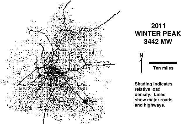
Figure 2.1 Map of electrical demand for a major U.S. city shows where the total demand of more than 2,000 MW peak is located. Degree of shading indicates electric load distribution. The T&D system must cover the region with sufficient capacity at every location to meet the consumer needs there.
Beyond the need to deliver power to the consumer, the utility’s T&D system must also deliver it in ready-to-use form - at the utilization voltage required for electrical appliances and equipment, and free of large voltage fluctuations, high levels of harmonics or transient electrical disturbances (Engel et al., 1992).
Most electrical equipment in the United States is designed to operate properly when supplied with 60 cycle alternating current at between 114 and 126 volts, a plus or minus five percent range centered on the nominal utilization voltage of 120 volts (RMS average of the alternating voltage). In many other countries, utilization standards vary from 230 to slightly over 250 volts, at either 50 or 60 cycles AC. 2 But regardless of the utilization voltage, a utility must maintain the voltage provided to each consumer within a narrow range centered within the voltages that electric equipment is designed to tolerate.
2 Power is provided to consumers in the United States by reversed alternating current legs (+120 volts and -120 volts wire to ground). This scheme provides 240 volts of power to any appliance that needs it, but for purposes of distribution engineering and performance, acts like only 120 volt power.
A ten- percent range of delivery voltage throughout a utility's service area may be acceptable, but a ten- percent range of fluctuation in the voltage supplied to any one consumer is not. An instantaneous shift of even three percent in voltage causes a perceptible (and to some people, disturbing) flicker in electric lighting. More importantly, voltage fluctuations can cause erratic and undesirable behavior of some electrical equipment.
Thus, whether high or low within the allowed range, the delivery voltage of any one consumer must be maintained at about the same level all the time -normally within a range of three to six percent - and any fluctuation must occur slowly. Such stable voltage can be difficult to obtain, because the voltage at the consumer end of a T&D system varies inversely with electric demand, falling as the demand increases, rising as it decreases. If this range of load fluctuation is too great, or if it happens too often, the consumers may consider it poor service.
Thus, a T&D system’s mission is to:
1. Cover the service territory, reaching all consumers
2. Have sufficient capacity to meet the peak demands of its consumers
3. Provide highly reliable delivery to its consumers
4. Provide stable voltage quality to its consumers
And of course, above everything else, achieve these four goals at the lowest cost possible.
2.3 THE LAWS OF T&D
The complex interaction of a T&D system is governed by a number of physical laws relating to the natural phenomena that have been harnessed to produce and move electric power. These interactions have created a number of “truths” that dominate the design of T&D systems:
1. It is more economical to move power at high voltage. The higher the voltage, the lower the costs per kilowatt to move power any distance.
2. The higher the voltage, the greater the capacity and the greater the cost of otherwise similar equipment. Thus, high voltage lines, while potentially economical, cost a great deal more than low voltage lines, but have a much greater capacity. They are only economical in practice if they can be used to move a lot of power in one block - they are the giant economy size, but while always giant, they are only economical if one truly needs the giant size.
3. Utilization voltage is useless for the transmission of power. The 120/240 volt single-phase utilization voltage used in the United States, or even the 250 volt/416 volt three-phase used in European systems is not equal to the task of economically moving power more than a few hundred yards. The application of these lower voltages for anything more than very local distribution at the neighborhood level results in unacceptably high electrical losses and high costs.
4. It is costly to change voltage level - not prohibitively so, for it is done throughout a power system (that’s what transformers do) -but voltage transformation is a major expense, which does nothing to move the power any distance in and of itself.
5. Power is more economical to produce in very large amounts. There is a significant economy of scale in generation, notwithstanding the claims by advocates of modern distributed generators. Large generators produce power more economically than small ones. Thus, it is most efficient to produce power at a few locations utilizing large generators.3
6. Power must be delivered in relatively small quantities at low (120 to 250 volt) voltage level. The average consumer has a total demand equal to only 1/10,000th or 1/100,000th of the output of a large generator.
An economical T&D system builds upon these concepts. It must “pick up” power at a few, large sites (generating plants), and deliver it to many, many more small sites (consumers). It must somehow achieve economy by using high voltage, but only when power flow can be arranged so that large quantities are moved simultaneously along a common path (line). Ultimately, power must be subdivided into “house- or business-sized” quantities, reduced to utilization voltage, and routed into each business and home via equipment whose compatibility with individual consumer needs means it will be relatively inefficient compared to the system as a whole. Regardless, this is the mission assigned to the retail power delivery system, what traditionally was called the “distribution system.”
3 The issue is more complicated than just a comparison of the cost of big versus small generation, as will be addressed later in this book. In some cases, distributed generation provides the lowest cost overall, regardless of the economy of scale, due to constraints imposed by the T&D system. Being close to the consumers, distributed generation does not carry with it the costs of adding T&D facilities to move the power from generation site to consumer. Often this is the margin of difference, as will be discussed later in this book.
Hierarchical Voltage Levels
The overall concept of a power delivery system layout that has evolved to best handle these needs and “truths” is one of hierarchical voltage levels as shown in Figures 2.2 and 2.3. As power is moved from generation (large bulk sources) to consumer (small demand amounts) it is first moved in bulk quantity at high voltage - this makes particular sense since there is usually a large bulk amount of power to be moved out of a large generating plant. As power is dispersed throughout the service territory, it is gradually moved down to lower voltage levels, where it is moved in ever smaller amounts (along more separate paths) on lower capacity equipment until it reaches the consumers. The key element is a “lower voltage and split” concept.
Thus, in Figure 2.3, the 3 kW used by a particular consumer -- Mrs. Watts at 412 Oak Street in Metropolis City - might be produced at a 800 MW power plant more than three hundred miles to the north. Her power is moved as part of a 750 MW block of wholesale from plant to city on a 345 kV transmission line, to a switching substation. Here, the voltage is lowered to 138 kV through a 345 to 138 kV transformer, and immediately after that, this large block is split into five separate smaller portions in the switching substation’s bus work. Each of these five parts, roughly 150 MW each, is routed onto a transmission line leaving that substation.
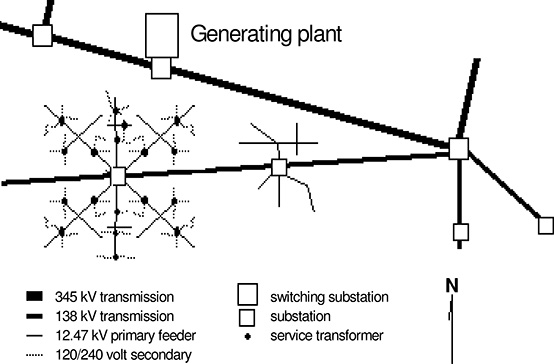
Figure 2.2 A power system is structured in a hierarchical manner with various voltage levels. A key concept is “lower voltage and split” which is done from three to five times during the course of power flow from generation to consumer.
Now part of one of these smaller blocks of power, Mrs. Watts’s electricity is routed to her side of Metropolis on a 138 kV transmission line that snakes 20 miles through the northern part of the city. Ultimately this line connects to another switching substation on the south side of the city. Along the way, it feeds power to several distribution substations along its route,4 among which it feeds 40 MW into the particular substation that serves Mrs. Watts’s neighborhood as well as others around that. Here, her power is run through a 138-kV to 12.47kV distribution transformer. At the low side of that substation transformer, at 12.47 kV (the primary distribution voltage) the 40 MW is split into six parts, each about 7 MW, with each 7 MVA part routed onto a different distribution feeder. Mrs. Watts’s power flows along one particular feeder for two miles, until it gets to within a few hundred feet of her home. Here, a much smaller amount of power, 50 kVA (sufficient for perhaps ten homes), is routed to a service transformer, one of several hundred scattered up and down the length of the feeder.
Once on the service transformer Mrs. Watts's power and that of her neighbors is lowered to utilitization voltage, the voltage at which the utility’s customers will use the power. In this case that is 120/240 volts (208 V phase to phase). As it emerges, from the service transformer, her power is routed onto the secondary system, operating at that 120/240 volt level (250/416 volts in Europe and many other countries). The secondary wiring splits the 50 kVA into small blocks of power, each about 5 kVA, and routes one of these to Mrs. Watts’s home along a secondary conductor to her service drops - the wires leading directly to her house.
Over the past one hundred years, this hierarchical system structure has proven a most effective way to move and distribute power from a few large generating plants to a widely dispersed consumer base. Neglecting light variations in design and operating practice from one utility to another, all power delivery systems are like this. The key element in this structure is the “reduce voltage and split” function - a splitting of the power flow being done simultaneously with a reduction in voltage. Usually, this happens between three and five times as power makes its way from generator to consumers.
2.4 LEVELS OF THE T&D SYSTEM
As a consequence of this hierarchical structure, a power delivery system can be thought of very conveniently to be composed of several distinct levels of equipment, as illustrated in Figure 2.3. Each level consists of many units of fundamentally similar equipment, doing roughly the same job, but located in different parts of the system. For example, all of the distribution substations are planned and designed in the same manner and do roughly the same job. Likewise all feeders are similar in equipment type, layout, and mission, and all service transformers have the same basic mission and are designed with similar planning goals and to similar engineering standards.
4 Transmission lines whose sole or major function is to feed power to distribution substations are often referred to as “sub-transmission” lines.
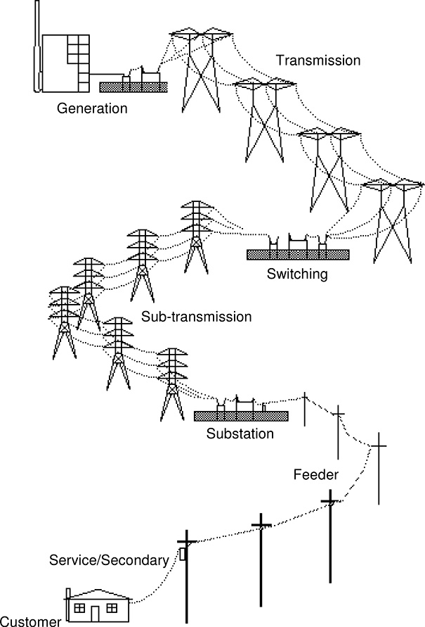
Figure 2.3 A T&D system consists of several levels of power delivery equipment, each feeding the one below it in an unbroken chain that delivers power to Mrs. Watts’ home.
Power can be thought of as flowing “down” through these levels, on its way from power production to consumer. As it moves from the generation plants (system level) to the consumer, the power travels through the transmission level, to the sub-transmission level, to the substation level, through the primary feeder level, and onto the secondary service level, where it finally reaches the consumer.
Each level takes power from the next higher level in the system and delivers it to the next lower level in the system. While each level varies in the types of equipment it has, its characteristics, mission, and manner of design and planning, all share several common characteristics:
• Each level is fed power by the one above it, in the sense that the next higher level is electrically closer to the generation.
• Both the nominal voltage level and the average capacity of equipment drops from level to level, as one moves from generation to consumer. Transmission lines operate at voltages of between 69 kV and 1,100 kV and have capacities between 50 and 2,000 MW. By contrast, distribution feeders operate between 2.2 kV and 34.5 kV and have capacities somewhere between 2 and 35 MW.
• Each level has many more pieces of equipment in it than the one above. A system with several hundred thousand consumers might have fifty transmission lines, one hundred substations, six hundred feeders, and forty thousand service transformers.
• As a result, the net capacity of each level (number of units times average size) increases as one moves toward the consumer. A power system might have 4,500 MVA of substation capacity but 6,200 MVA of feeder capacity and 9,000 MVA of service transformer capacity installed.5
• Reliability drops as one moves closer to the consumer. A majority of service interruptions are a result of failure (either due to aging or to damage from severe weather) of transformers, connectors, or conductors very close to the consumer, as shown in Figure 2.4.
5 This greater-capacity-at-every-level is deliberate and required both for reliability reasons and to accommodate coincidence of load, which will be discussed in Chapter 3.
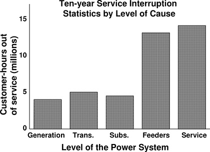
Figure 2.4 Ten years of consumer interruptions for a large electric system, grouped by level of cause. Interruptions due to generation and transmission often receive the most attention because they usually involve a large number of consumers simultaneously. However, such events are rare whereas failures and interruptions at the distribution level create a constant background level of interruptions.
Table 2.1 gives statistics for a typical system. The net effect of the changes in average size and number of units is that each level contains a greater total capacity than the level above it. The service transformer level in any utility system has considerably more installed capacity (number of units times average capacity) than the feeder system or the substation system. Total capacity increases as one heads toward the consumer because of non-coincidence of peak load (which will be discussed in Chapter 3) and for reliability purposes.
Table 2.1 Equipment Level Statistics for a Medium-Sized Electric System

The (Wholesale) Transmission Level
The transmission system is a network of three-phase lines operating at voltages generally between 115 kV and 765 kV. Capacity of each line is between 50 MVA and 2,000 MVA. The term “network” means that there is more than one electrical path between any two points in the system (Figure 2.5). Networks are laid out in this manner for reasons of reliability and operating flow--if any one element (line) fails, there is an alternate route and power flow is (hopefully) not interrupted.
In addition to their function in moving power, portions of the transmission system, the largest elements, namely its major power delivery lines, are designed, at least in part, for stability needs. The transmission grid provides a strong electrical tie between generators, so that each can stay synchronized with the system and with the other generators. This arrangement allows the system to operate and to function evenly as the load fluctuates and to pick up load smoothly if any generator fails - what is called stability of operation. A good deal of the equipment put into transmission system design, and much of its cost, is for these stability reasons, not solely or even mainly, for moving power.
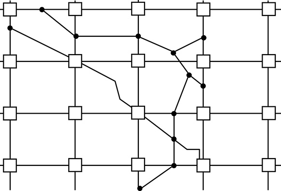
Figure 2.5 A network is an electrical system with more than one path between any two points, meaning that (if properly designed) it can provide electrical service even if any one element fails.
The Sub-transmission Level
The sub-transmission lines in a system take power from the transmission switching stations or generation plants and deliver it to substations along their routes. A typical sub-transmission line may feed power to three or more substations. Often, portions of the transmission system, bulk power delivery lines, lines designed at least in part for stability as well as power delivery needs to do this too. The distinction between transmission and sub-transmission lines becomes rather blurred.
Normally, sub-transmission lines are in the range of capacity of 30 MVA up to perhaps 250 MVA, operating at voltages from 34.5 kV to as high as 230 kV. With occasional exceptions, sub-transmission lines are part of a network grid - they are part of a system in which there is more than one route between any two points. Usually, at least two sub-transmission routes flow into any one substation, so that feed can be maintained if one fails.6
The Substation Level
Substations, the meeting point between the transmission grid and the distribution feeder system, are where a fundamental change takes place within most T&D systems. The transmission and sub-transmission systems above the substation level usually form a network, as discussed above, with more than one power flow path between any two parts. But from the substation on to the consumer, arranging a network configuration would simply be prohibitively expensive. Thus, most distribution systems are radial - there is only one path through the other levels of the system.
Typically, a substation occupies an acre or more of land on which the necessary substation equipment is located. Substation equipment consists of high and low voltage racks and busses for the power flow, circuit breakers for both the transmission and distribution level, metering equipment, and the “control house,” where the relaying, measurement, and control equipment is located. But the most important equipment, what gives this substation its capacity rating, are the substation transformers. These transformers convert the incoming power from transmission voltage levels to the lower primary voltage for distribution.
Individual substation transformers vary in capacity, from less than 10 MVA to as much as 150 MVA. They are often equipped with tap-changing mechanisms and control equipment to vary their winding ratio so that they maintain the distribution voltage within a very narrow range, regardless of larger fluctuations on the transmission side. The transmission voltage can swing by as much as 5%, but the distribution voltage provided on the low side of the transformer stays within a narrow band, perhaps only ± .5%.
6 Radial feed - only one line - is used in isolated, expensive, or difficult transmission situations, but for reliability reasons is not recommended.
Very often, a substation will have more than one transformer. Two is a common number, four is not uncommon, and occasionally six or more are located at one site. Having more than one transformer increases reliability. In an emergency, a transformer can handle a load much over its rated load for a brief period (e.g., perhaps up to 140% of rating for up to four hours). Thus, the T&D system can pick up the load of the outaged portions during brief repairs and in emergencies.
Equipped with one to six transformers, substations range in “size” or capacity from as little as five MVA for a small, single-transformer substation, serving a sparsely populated rural area, to more than 400 MVA for a truly large six-transformer station, serving a very dense area within a large city.
Often T&D planners will speak of a transformer unit, which includes the transformer and all the equipment necessary to support its use - “one fourth of the equipment in a four-transformer substation.” This is a much better way of thinking about and estimating cost for equipment in T&D plans. While a transformer itself is expensive (between $50,000 and $1,000,000); the buswork, control, breakers, and other equipment required to support its use can double or triple that cost. Since that equipment is needed in direct proportion to the transformer’s capacity and voltage, and since it is needed only because a transformer is being added, it is normal to associate it with the transformer as a single planning unit. Add the transformer and add the other equipment along with it.
Substations consist of more equipment and involve more costs than just the electrical equipment. The site has to be purchased and prepared. Preparation is not trivial. The site must be excavated, a grounding mat - wires running under the substation to protect against an inadvertent flow during emergencies - laid down, and foundations and control ducting for equipment must be installed. Transmission towers to terminate incoming transmission must be built. Feeder getaways - ducts or lines to bring power out to the distribution system - must be added.
The Feeder Level
Feeders, typically either overhead distribution lines mounted on wooden poles or underground buried or ducted cable sets, route the power from the substation throughout its service area. Feeders operate at the primary distribution voltage. The most common primary distribution voltage in use throughout North America is 12.47 kV, although anywhere from 4.2 kV to 34.5 kV is widely used. Worldwide, there are primary distribution voltages as low as 1.1 kV and as high as 66 kV. Some distribution systems use several primary voltages - for example 23.9 kV, 13.8 kV and 4.16 kV.
A feeder is a small transmission system in its own right, distributing between 2 MVA to more than 30 MVA, depending on the conductor size and the distribution voltage level. Normally between two and 12 feeders emanate from any one substation, in what has been called a dendrillic configuration - repeated branching into smaller branches as the feeder moves out from the substation toward the consumers. In combination, all the feeders in a power system constitute the feeder system (Figure 2.6). An average substation has between two and eight feeders, and can vary between one and forty feeders.
Figure 2.6 Distribution feeders route power away from the substation, as shown (in idealized form - configuration is never so evenly symmetric in the real world) for two substations. Positions of switches make the system electrically radial, while parts of it are physically a network. Shown here are two substations, each with four feeders.
The main, three-phase trunk of a feeder is called the primary trunk and may branch into several main routes, as shown in the diagram on the next page. These main branches end at open points where the feeder meets the ends of other feeders - points at which a normally open switch serves as an emergency tie between two feeders.
Additionally, normally closed switches in several switchable elements will divide each feeder. During emergencies, segments can be re-switched to isolate damaged sections and route power around outaged equipment to consumers who would otherwise have to remain out of service until repairs were made.
By definition, the feeder consists of all primary voltage level segments between the substations and an open point (switch). Any part of the distribution level voltage lines - three-phase, two-phase, or single-phase - that is switchable is considered part of the primary feeder. The primary trunks and switchable segments are usually built using three phases. The largest size of distribution conductor (typically this is about 500-600 MCM conductor, but a conductor over 1,000 MCM is not uncommon, and one of the authors designed and built a feeder with a 2,000 MCM conductors) being used for reasons other than just maximum capacity (e.g., contingency switching needs). Often a feeder has excess capacity because it needs to provide back up for other feeders during emergencies.
The vast majority of distribution feeders used worldwide and within the United States are overhead construction, wooden pole with wooden crossarm or post insulators. Only in dense urban areas, or in situations where esthetics are particularly important, can the higher cost of underground construction be justified. In this case, the primary feeder is built from insulated cable, which is pulled through concrete ducts that are first buried in the ground. Underground feeder costs are three to ten times that of overhead costs.
Many times, however, the first several hundred yards of an overhead primary feeder are built underground even if the system is overhead. This underground portion is used as the feeder get-away. Particularly at large substations, the underground get-away is dictated by practical necessity, as well as by reliability and esthetics. At a large substation, ten or twelve 3-phase, overhead feeders leaving the substation mean from 40 to 48 wires hanging in mid-air around the substation site, with each feeder needing the proper spacing for electrical insulation, safety, and maintenance.
One significant aging infrastructure issue is that at many large-capacity substations in a tight location, there is simply not enough overhead space for enough feeders to be routed out of the substation. Even if there is, the resulting tangle of wires looks unsightly, and perhaps most importantly, is potentially unreliable. One broken wire falling in the wrong place can disable a lot of power delivery capability. The solution to this dilemma is the underground feeder get-away, usually consisting of several hundred yards of buried, ducted cable that takes the feeder out to a riser pole, where it is routed above ground and connected to overhead wires. Very often, this initial underground link sets the capacity limit for the entire feeder. The underground cable ampacity is the limiting factor for the feeder's power transmission.
The Lateral Level
Laterals are short stubs or line-segments that branch off the primary feeder and represent the final primary voltage part of the power's journey from the substation to the consumer. A lateral is directly connected to the primary trunk and operates at the same nominal voltage. A series of laterals tap off the primary feeder as it passes through a community, each lateral routing power to a few dozen homes.
Normally, laterals do not have branches, and many laterals are only one or two-phase. All three phases are used only if a relatively substantial amount of power is required, or if three-phase service must be provided to some of the consumers. Normally, single and two-phase laterals are arranged to tap alternately into different phases on the primary feeder. An attempt by the Distribution Planning Engineer to balance the loads as closely as possible is shown below.
Typically, laterals deliver from as little as 10 kVA for a small single-phase lateral, to as much as 2 MVA. In general, even the largest laterals use small conductors (relative to the primary size). When a lateral needs to deliver a great deal of power, the planner will normally use all three phases, with a relatively small conductor for each, rather than employ a single-phase and use a large conductor. This approach avoids creating a significant imbalance in loading at the point where the lateral taps into the primary feeder. Power flow, loadings and voltage are maintained in a more balanced state if the power demands of a “large lateral” are distributed over all three phases.
Laterals (wooden poles) are built overhead or underground. Unlike primary feeders and transmission lines, single-phase laterals are sometimes buried directly. In this case, the cable is placed inside a plastic sheath (that looks and feels much like a vacuum cleaner hose). A trench is dug, and the sheathed cable is unrolled into the trench and buried. Directly buried laterals are no more expensive than underground construction in many cases.
The Service Transformers
Service transformers lower voltage from the primary voltage to the utilization or consumer voltage, normally 120/240-volt two-leg service in most power systems throughout North America. In overhead construction, service transformers are pole mounted and single-phase, between 5-kVA and 166 -kVA capacity. There may be several hundred scattered along the trunk and laterals of any given feeder; since power can travel efficiently only up to about 200 feet at utilization voltage, there must be at least one service transformer located reasonably close to every consumer. In underground areas, service transformers may be located in underground vaults, or at ground level (pad-mounted).
Passing through these transformers, power is lowered in voltage once again, to the final utilization voltage (120/240 volts in the United States) and routed to the secondary system or directly to the consumers. In cases where the system is supplying power to large commercial or industrial consumers, or the consumer requires three-phase power, between two and three transformers may be located together in a transformer bank, and be interconnected in such a way as to provide multi-phase power. Several different connection schemes are possible for varying situations.
Padmount and vault-type service transformers provide underground service, as opposed to overhead pole-mounted service. The concept is identical to overhead construction, with the transformer and its associated equipment changed to accommodate incoming and outgoing lines that are underground.
The Secondary and Service Level
Secondary circuits fed by the service transformers route power at utilization voltage within very close proximity to the consumer. Usually this is an arrangement in which each transformer serves a small radial network of utilization voltage secondary and service lines. These lead directly to the meters of consumers in the immediate vicinity.
At most utilities, the layout and design of the secondary level is handled through a set of standardized guidelines and tables. Engineering technicians use these and clerks to produce work orders for the utilization voltage level equipment. In the United States, the vast majority of this system is single-phase. In European systems, much of the secondary is 3-phase, particularly in urban and suburban areas.
What is Transmission and What is Distribution?
Definitions and nomenclature defining “transmission” and “distribution” vary greatly among different countries, companies, and power systems. Generally, four types of distinction between the two are made, only three of which are dealt with it this book:
By economic societal function: As noted in Chapter 1, in the United States, the wholesale transmission, or grid level, is defined and operated differently from local power delivery, by Federal mandate. This distinction is not addressed in this book.
By voltage class: transmission is anything above 34.5 kV; primary distribution is anything below that but above the utilization voltage.
By function: distribution includes all utilization voltage equipment, plus all lines that feed power to service transformers.
By configuration: transmission is nearly always a network or heavily looped circuits. Distribution is nearly always radial or a simple loop scheme.
Generally, the last three definitions apply simultaneously since in most utility systems any transmission above 34.5 kV is configured as a network and does not feed service transformers directly. On the other hand, all distribution is radial, built of only 34.5 kV or below, and does feed service transformers. Substations - the meeting places of transmission lines (incoming) and distribution lines (outgoing) - are often included in one or the other category, and sometimes are considered as separate entities.
2.5 UTILITY DISTRIBUTION EQUIPMENT
The preceding section made it clear that a power delivery system is a very complex entity, composed of thousands, perhaps even millions, of components, which function together as a T&D system. Each unit of equipment has only a small part to play in the system, and is only a small part of the cost, yet each is critical for satisfactory service to at least one or more consumers or it would not be included in the system.
T&D system planning is complex because each unit of equipment influences the electrical behavior of its neighbors. It must be designed to function well in conjunction with the rest of the system, under a variety of different conditions, regardless of shifts in the normal pattern of loads or the status of equipment nearby. While the modeling and analysis of a T&D system can present a significant challenge, individually its components are relatively simple to understand, engineer, and plan. In essence, there are only two major types of equipment that perform the power delivery function:
1. Transmission and distribution lines move power from one location to another
2. Transformers change the voltage level of the power
Added to these three basic equipment types are two categories of equipment used for a very good reason:
1. Protective equipment which provides safety and “fail safe” operation.
2. Voltage regulation equipment that is used to maintain voltage within an acceptable range as the load changes.
3. Monitoring and control equipment that measures equipment and system status feeds this information to control systems so that the utility knows what the system is doing and can control it.
Transmission and Distribution Lines
By far the most omnipresent part of the power distribution system is the portion devoted to actually moving the power flow from one point to another. Transmission lines, sub-transmission lines, feeders, laterals, secondary and service drops, all consist of electrical conductors, suitably protected by isolation (transmission towers, insulator strings, and insulated wrappings) from voltage leakage and ground contact. It is this conductor that carries the power from one location to another.
Electrical conductors are available in various capacity ranges, with capacity generally corresponding to the metal cross section (other things being equal, thicker wire carries more power). Conductors can be all steel (rare, but used in some locations where winter ice and wind loadings are quite severe), all aluminum, or copper, or a mixture of aluminum and steel. Underground transmission can use various types of high-voltage cable. Line capacity depends on the current-carrying capacity of the conductor or the cable, the voltage, the number of phases, and constraints imposed by the line's location in the system.
The most economical method of handling a conductor is to place it overhead, supported by insulators on wooden poles or metal towers suitably clear of interference or contact with persons or property. However, underground construction, while generally more costly, avoids esthetic intrusion of the line and provides some measure of protection from weather. It also tends to reduce the capacity of a line slightly due to the differences between underground cable and overhead conductor. Suitably wrapped with insulating material in the form of underground cable, the cable is placed inside concrete or metal ducts or surrounded in a plastic sheath.
Transmission/sub-transmission lines are always 3-phase. There are three separate conductors for the alternating current, sometimes with a fourth neutral (un-energized) wire. Voltage is measured between phases. A 12.47 kV distribution feeder has an alternating current voltage (RMS) of 12,470 volts as measured between any two phases. Voltage between any phase and ground is 7,200 volts (12.47 divided by the square root of three). Major portions of a distribution system - trunk feeders - are as a rule built as three-phase lines, but lower-capacity portions may be built as either two-phase, or single-phase.7
Regardless of type or capacity, every electrical conductor has impedance (a resistance to electrical flow through it) that causes voltage drop and electrical losses whenever it is carrying electric power. Voltage drop is a reduction in the voltage between the sending and receiving ends of the power flow. Losses are a reduction in the net power, and are proportional to the square of the power. Double the load and the losses increase by four. Thus, 100 kilowatts at 120 volts might go in one end of a conductor, only to emerge at the other as 90 kilowatts at 114 volts at the other end. Both voltage drop and losses vary in direct relation to load - within very fine limits if there is no load, there are no losses or voltage drop. Voltage drop is proportional to load. Double the load and voltage drop doubles. Losses are quadratic, however. Double the load and losses quadruple.
7 In most cases, a single-phase feeder or lateral has two conductors: the phase conductor and the neutral.
Transformers
At the heart of any alternating power system are transformers. They change the voltage and current levels of the power flow, maintaining (except for a very small portion of electrical losses), the same overall power flow. If voltage is reduced by a factor of ten from the high to low side, then Current is multiplied by ten, so that their overall product (Voltage times Current equals Power) is constant in and out.
Transformers are available in a diverse range of types, sizes, and capacities. They are used within power systems in four major areas:
1. At power plants, where power which is minimally generated at about 20,000 volts is raised to transmission voltage (100,000 volts or higher),
2. At switching stations, where transmission voltage is changed (e.g., from 345,000 volts to 138,000 volts before splitting onto lower voltage transmission lines),
3. At distribution substations, where incoming transmission-level voltage is reduced to distribution voltage for distribution (e.g., 138 kV to 12.47 kV),
4. And at service transformers, where power is reduced in voltage from the primary feeder voltage to utilization level (12.47 kV to 120/240 volts) for routing into consumers’ homes and businesses.
Larger transformers are generally built as three-phase units, in which they simultaneously transform all three phases. Often these larger units are built to custom or special specifications, and can be quite expensive - over $3,000,000 per unit in some cases. Smaller transformers, particularly most service transformers, are single-phase - it takes three installed side by side to handle a full three-phase line’s power flow. They are generally built to standard specifications and bought in quantity.
Transformers experience two types of electrical losses - no-load losses (often called core, or iron, losses) and load-related losses.
No-load losses are electrical losses inherent in operating the transformer -due to its creation of a magnetic field inside its core. They occur simply because the transformer is connected to an electrical power source. They are constant, regardless of whether the power flowing through the transformer is small or large. No-load losses are typically less than one percent of the nameplate rating. Only when the transformer is seriously overloaded, to a point well past its design range, will the core losses change (due to magnetic saturation of the core).
Load-related losses are due to the current flow through the transformer's impedance and correspond very directly with the level of power flow. Like those of conductors and cables they are proportional to current squared or quadrupling whenever power flow doubles. The result of both types of losses is that a transformer's losses vary as the power transmitted through it varies, but always at or above a minimum level set by the no-load losses.
Switches
Occasionally, it is desirable to be able to vary the connection of line segments within a power delivery system, particularly in the distribution feeders. Switches are placed at strategic locations so that the connection between two segments can be opened or closed. Switches are planned to be normally closed (NC) or normally open (NO), as was shown in Figure 2.6.
Switches vary in their rating (how much current they can vary) and their load break capacity (how much current they can interrupt or switch off), with larger switches being capable of opening a larger current. They can be manually, automatically, or remotely controlled in their operation.
Protection
When electrical equipment fails, for example if a line is knocked down during a storm, the normal function of the electrical equipment is interrupted. Protective equipment is designed to detect these conditions and isolate the damaged equipment, even if this means interrupting the flow of power to some consumers. Circuit breakers, sectionalizers, and fused disconnects, along with control relays and sensing equipment, are used to detect unusual conditions and interrupt the power flow whenever a failure, fault, or other unwanted condition occurs on the system.
These devices and the protection engineering required to apply them properly to the power system are not the domain of the utility planners and will not be discussed here. Protection is vitally important, but the planner is sufficiently involved with protection if he or she produces a system design that can be protected within standards, and if the cost of that protection has been taken into account in the budgeting and planning process. Both of these considerations are very important.
Protection puts certain constraints on equipment size and layout - for example, in some cases a very large conductor is too large (because it would permit too high a short circuit current) to be protected safely by available equipment and cannot be used. In other cases, long feeders are too long to be protected (because they have too low a short circuit current at the far end). A good deal of protective equipment is quite complex, containing sensitive electro-mechanical parts (many of which move at high speeds and in a split-second manner), and depending on precise calibration and assembly for proper function. As a result, the cost of protective equipment and control and the cost of its maintenance are often significant. Differences in protection cost can make the deciding difference between two plans.
Voltage Regulation
Voltage regulation equipment includes line regulators and line drop compensators, as well as tap changing transformers. These devices vary their turns-ratio (ratio of voltage in to voltage out) to react to variations in voltage drop. If voltage drops, they raise the voltage; if voltage rises, they reduce it to compensate. Properly used, they can help maintain voltage fluctuation on the system within acceptable limits, but they can only reduce the range of fluctuation, not eliminate it altogether.
Capacitors
Capacitors are a type of voltage regulation equipment. By correcting power factor they can improve voltage under many heavy loads (hence large voltage drop) cases. Power factor is a measure of how well voltage and current in an alternating system are in step with one another. In a perfect system, voltage and current would alternately cycle in conjunction with one another - reaching a peak, then reaching a minimum, at precisely the same times. But on distribution systems, particularly under heavy load conditions, current and voltage fall out of phase. Both continue to alternate 60 times a second, but during each cycle voltage may reach its peak slightly ahead of current - there is a slight lag of current versus voltage, as shown in Figure 2.7.
It is the precise, simultaneous peaking of both voltage and current that delivers maximum power. If out of phase, even by a slight amount, effective power drops, as does power factor - the ratio of real (effective) power to the maximum possible power, if voltage and current were locked in step.
Power engineers refer to a quantity called VARs (Volt-Amp Reactive) that is caused by this condition. Basically, as power factors worsen (as voltage and current fall farther apart in terms of phase angle) a larger percentage of the electrical flow is VARs, and a smaller part is real power. The frustrating thing is that the voltage is still there, and the current is still there, but because of the shift in their timing, they produce only VARS, not power. The worse the power factor, the higher the VAR content. Poor power factor creates considerable cost and performance consequences for the power system: a large conductor is still required to carry the full level of current even though power delivery has dropped. And because current is high, the voltage drop is high, too, further degrading quality of service.
Unless one has worked for some time with the complex variable mathematics associated with AC power flow analysis, VARs are difficult to picture. A useful analogy is to think of VARs as “electrical foam.” If one tried to pump a highly carbonated soft drink through a system of pipes, turbulence in the pipes, particularly in times of high demand (high flow) would create foam. The foam would take up room in the pipes, but contribute little value to the net flow - the equivalent of VARs in an electrical system.
Poor power factor has several causes. Certain types of loads create VARs -loads that cause a delay in the current with respect to voltage as it flows through them. Among the worst offenders are induction motors - particularly small ones as almost universally used for blowers, air conditioning compressors, and the powering of conveyor belts and similar machinery. Under heavy load conditions, voltage and current can get out of phase to the point that the power factor can drop below 70%. Additionally, transmission equipment itself can often create this lag and “generate” a poor power factor.
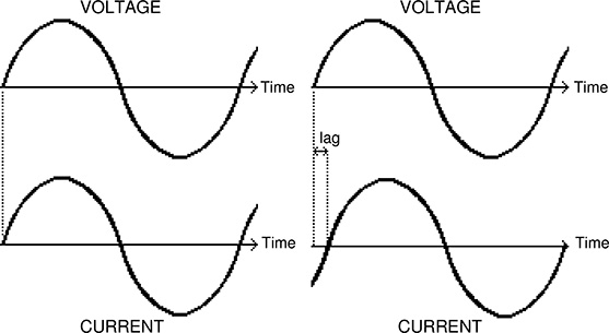
Figure 2.7 Current and voltage in phase deliver maximum power (left). If current and voltage fall out of phase (right), actual power delivered drops by very noticeable amounts -- the power factor falls.
Capacitors correct the poor power factor. They “inject” VARs into a T&D line to bring power factor close to 1.0, transforming VAR flow back into real power flow, regaining the portion of capacity lost to poor power factor. Capacitors can involve considerable cost depending on location and type. They tend to do the most good if put on the distribution system, near the consumers, but they cost a great deal more in those locations than if installed at substations.
2.6 T&D COSTS
A T&D system can be expensive to design, build, and operate. Equipment at every level incurs two types of costs. Capital costs include the equipment and land, labor for site preparation, construction, assembly and installation, and any other costs associated with building and putting the equipment into operation. Operating costs include labor and equipment for operation, maintenance and service, taxes and fees, as well as the value of the power lost to electrical losses. Usually, capital costs are a one-time cost (once it’s built, the money's been spent). Operating costs are continuous or periodic.
Electrical losses vary depending on load and conditions. While these losses are small by comparison to the overall power being distributed (seldom more than 8%), they constitute a very real cost to the utility. The present worth of the lifetime losses through a major system component such as a feeder or transformer can be a significant factor impacting its design and specification, often more than the original capital cost of the unit. Frequently, a more costly type of transformer will be selected for a certain application because its design leads to overall savings due to lower losses. Or a larger capacity line (larger conductor) will be used when really needed due to capacity requirements, purely because the larger conductor will incur lower cost losses.
Cumulatively, the T&D system represents a considerable expense. While a few transmission lines and switching stations are composed of large, expensive, and purpose-designed equipment, the great portion of the sub-transmission-substation-distribution system is built from “small stuff” -commodity equipment bought mostly “off the shelf” to standard designs. Individually inexpensive, they amount to a significant cost when added together.
Transmission Costs
Transmission line costs are based on a per-mile cost and a termination cost at either end of the line associated with the substation at which it is terminated. Costs can run from as low as $50,000/mile for a 46 kV wooden pole sub-transmission line with perhaps 50 MVA capacity ($1 per kVA-mile) to over $1,000,000 per mile for a 500 kV double circuit construction with 2,000 MVA capacity ($.5/kVA-mile).
Substation Costs
Substation costs include all the equipment and labor required to build a substation, including the cost of land and easements/ROW. For planning purposes, substations can be thought of as having four costs:
1. Site cost - the cost of buying the site and preparing it for a substation, including the cost of all legal work required to gain permissions and licenses (this can sometimes exceed the cost of the land).
2. Transmission cost - the cost of terminating the incoming sub-transmission lines at the site.
3. Transformer cost - the transformer and all metering, control, oil spill containment, fire prevention, cooling, noise abatement, and other related equipment, along with buswork, switches, metering, relaying, and breakers associated with this type of transformer, and their installation.
4. Feeder buswork/Get-away costs - the cost of beginning distribution at the substation, includes getting feeders out of the substation.
To expedite planning, estimated costs of feeder buswork and get-aways are often folded into the transformer costs. The feeders to route power out of the substation are needed in conjunction with each transformer and in direct proportion to the transformer capacity installed, so that their cost is sometimes considered together with the transformer as a single unit. Regardless, the transmission, transformer, and feeder costs can be estimated fairly accurately for planning purposes.
Cost of land is another matter entirely. Site and easements or ROW into a site have a cost that is a function of local land prices, which vary greatly depending on location and real estate markets. Site preparation includes the cost of preparing the site which includes grading, grounding mat, foundations, buried ductwork, control building, lighting, fence, landscaping, and an access road.
Substation costs vary greatly depending on type, capacity, local land prices and other variable circumstances. In rural settings where load density is quite low and minimal capacity is required, a substation may involve a site of only several thousand square feet of fenced area. This single area includes a single incoming transmission line (69 kV), one 5 MVA transformer; fusing for all fault protection; and all “buswork” built with wood poles and conductor, for a total cost of perhaps no more than $90,000. The substation would be applied to serve a load of perhaps 4 MW, for a cost of $23/kW. This substation in conjunction with the system around it would probably provide service with about ten hours of service interruptions per year under average conditions.
However, a typical substation built in most suburban and urban settings would be fed by two incoming 138 kV lines feeding two 40 MVA, 138 kV to 12.47 kV transformers. These transformers would each feed a separate low side (12.47 kV) bus, each bus with four outgoing distribution feeders of 9 MVA peak capacity each, and a total cost of perhaps $2,000,000. Such a substation’s cost could vary from between about $1.5 million and $6 million, depending on land costs, labor costs, the utility equipment and installation standards, and other special circumstances. In most traditional vertically integrated, publicly regulated electric utilities, this substation would have been used to serve a peak load of about 60 MVA (75% utilization of capacity), meaning that at its nominal $2,000,000 cost works out to $33/kW. In a competitive industry, with tighter design margins and proper engineering measures taken beforehand, this could be pushed to a peak loading of 80 MVA (100% utilization, $25/kW). This substation and the system around it would probably provide service with about two to three hours of service interruptions per year under “normal,” average conditions.
Feeder System Costs
The feeder system consists of all the primary distribution lines, including three-phase trunks and their lateral extensions. These lines operate at the primary distribution voltage - 23.9 kV, 13.8 kV, 12.47 kV, 4.16kV or whatever - and may be three-, two-, or single-phase construction as required. Typically, the feeder system is also considered to include voltage regulators, capacitors, voltage boosters, sectionalizers, switches, cutouts, fuses, and any intertie transformers (required to connect feeders of different voltage at tie points - for example: 23.9 and 12.47 kV) that are installed on the feeders (not at the substations or at consumer facilities).
As a rule of thumb, construction of three-phase overhead, wooden pole crossarm type feeders using a normal, large conductor (about 600 MCM per phase) at a medium distribution primary voltage (e.g., 12.47 kV) costs about $150,000/mile. However, cost can vary greatly due to variations in labor, filing and permit costs among utilities, as well as differences in design standards, and terrain. Where a thick base of topsoil is present, a pole can be installed by simply auguring a hole for the pole. In areas where there is rock close under the surface, holes have to be jack-hammered or blasted, and costs go up accordingly. It is generally less expensive to build feeders in rural areas than in suburban or urban areas. Thus, while $150,000 is a good average cost, a mile of new feeder construction could cost as little as $55,000 in some situations and as much as $500,000 in others.
A typical distribution feeder (three-phase, 12.47 kV, 600 MCM/phase) would be rated at a thermal (maximum) capacity of about 15 MVA and a recommended economic (design) peak loading of about 8.5 MVA peak, depending on losses and other costs. At $150,000/mile, this capacity rating gives somewhere between $10 to $15 per kW-mile as the cost for basic distribution line. Underground construction of a three-phase primary feeder is more expensive, requiring buried ductwork and cable, and usually works out to a range of $30 to $50 per kW-mile.
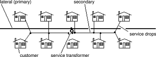
Figure 2.8 Here, a service transformer, fed from a distribution primary-voltage lateral, feeds in turn ten homes through a secondary circuit operating at utilization voltage.
Lateral lines, short primary-voltage lines working off the main three-phase circuit, are often single- or two-phase and consequently have lower costs but lower capacities. Generally, they are about $5 to $15 per kW-mile overhead, with underground costs of between $5 to $15 per kW-mile (direct buried) to $30 to $100 per kW-mile (ducted).
Cost of other distribution equipment, including regulators, capacitor banks and their switches, sectionalizers, line switches, etc., varies greatly depending on the specifics of each application. In general, the cost of the distribution system will vary from between $10 and $30 per kW-mile.
Service Level Costs
The service or secondary system consists of the service transformers that convert primary voltage to utilization voltage, the secondary circuits that operate at utilization voltage, and the service drops that feed power directly to each consumer. Without exception these are very local facilities, meant to move power no more than a few hundred feet at the very most and deliver it to the consumer “ready to use.”
Many electric utilities develop cost estimates for this equipment on a per-consumer basis. A typical service configuration might involve a 50 MVA pole-mounted service transformer feeding ten homes, as shown in Figure 2.8. Costs for this equipment might include:
Heavier pole & hardware for transformer application |
$250 |
50 kW transformer, mounting equipment, and installation |
$850 |
500 feet secondary (120/240 volt) single-phase @ $2/ft. |
$1,100 |
10 service drops including installation at $100 |
$1,100 |
$3,300 |
For a cost of about $330 per consumer, or about $66/kW of coincident load.
Maintenance and Operating Costs
Once put into service, T&D equipment must be maintained in sound, operating condition, hopefully in the manner intended and recommended by the manufacturer. This will require periodic inspection and service, and may require repair due to damage from storms or other contingencies. In addition, many utilities must pay taxes or fees for equipment (T&D facilities are like any other business property). Operating, maintenance, and taxes are a continuing annual expense.
It is very difficult to give any generalization of O&M&T costs, partly because they vary so greatly from one utility to another, but mostly because utilities account for and report them in very different ways. Frankly, the authors have never been able to gather a large number of comparable data sets from which to produce even a qualitative estimate of average O&M&T costs.8 With that caveat, a general rule of thumb: O&M&T costs for a power delivery system probably run between 1/8 and 1/30 of the capital cost, annually.
The Cost to Upgrade Exceeds the Cost to Build
One of the fundamental factors affecting design of T&D systems and management of an electric utility is that it costs more to upgrade equipment to a higher capacity than to build to that capacity in the original construction. For example, a 12.47 kV overhead, three-phase feeder with a 9 MW peak load capability (336 MCM phase conductor) might cost $240,000/mile to build ($26.66 per kW-mile). Building it with a 600 MCM conductor instead, for a capacity of 15 MVA, would cost in the neighborhood of $300,000 ($20/kW-mile).
8 For example, some utilities include part of O&M expenses in overhead costs, others do not. A few report repairs (including storm damage) as part of O&M, others accumulate major repair work separately. Others report parts of routine service (periodic rebuilding of breakers) as a type of capital cost because it extends equipment life or augments capacity. Others report all such work as O&M. Such differences are common among utilities.
However, upgrading an existing 336 MCM, 9 MW capacity line to 600 MCM and 15 MVA capacity could probably cost the utility at least $500,000/mile - over $83 per kW-mile for the additional capacity. It is more expensive because replacement entails removing the old conductor and installing a new conductor along with brackets, cross-arms, and other hardware required supporting the heavier new conductor. Another factor is that typically this work has to be done “hot” (i.e., with the feeder energized and feeding power to customers) which means the work must be undertaken with extreme care and following a number of safety-related procedure that require additional equipment and labor. By contrast the original construction is done cold – with the power turned off and no customers yet served by the circuit.
Thus, T&D planners have an incentive to look at their long-term needs carefully, and to "overbuild" against initial requirements if growth trends show future demand will be higher. The cost of doing so must be weighed against long-term savings, but often T&D facilities are built with considerable margin (50%) above existing load to allow for future load growth.
The very high cost per kW for upgrading a T&D system in place creates one of the best-perceived opportunities for DSM and DG reduction. Note that the capital cost/kW for the upgrade capacity in the example above ($33/kW) is nearly three times the cost of similar new capacity. Thus, planners often look at areas of the system where slow, continuing load growth has increased load to the point that local delivery facilities are considerably taxed, as areas where DSM and DG can deliver significant savings.
In some cases, distributed resources can reduce or defer significantly the need for T&D upgrades of the type described above. However, this does not assure significant savings for the situation is more complicated than an analysis of capital costs to upgrade may indicate. If the existing system (e.g., the 9 MW feeder) needs to be upgraded, then it is without a doubt highly loaded, which means its losses may be high, even off-peak. The upgrade to a 600 MCM conductor will cut losses 8,760 hours per year. Financial losses may drop by a significant amount, enough in many cases to justify the cost of the upgrade alone. The higher the annual load factor in an area, the more likely this is to occur, but it is often the case even when load factor is only 40%. However, DSM and in some cases DG also lowers losses, making the comparison quite involved, as will be discussed later in this book.
Electrical Losses Costs
Movement of power through any electrical device, be it a conductor, transformer, regulator or whatever, incurs a certain amount of electrical loss due to the impedance (resistance to the flow of electricity) of the device. These losses are a result of inviolable laws of nature. They can be measured, assessed, and minimized through proper engineering, but never eliminated completely.
Losses are an operating cost
Although losses do create a cost (sometimes a considerable one) it is not always desirable to reduce them as much as possible. Perhaps the best way to put them in proper perspective is to think of T&D equipment as powered by electricity - the system that moves power from one location to another runs on electric energy itself. Seen in this light, losses are revealed as what they are - a necessary operating expense to be controlled and balanced against other costs.
Consider a municipal water department, which uses electric energy to power the pumps that drive the water through the pipes to its consumers. Electricity is an acknowledged operating cost, one accounted for in planning, and weighed carefully in designing the system and estimating its costs. The water department could choose to buy highly efficient pump motors. Motors that command a premium price over standard designs but provide a savings in reduced electric power costs, use piping that is coated with a friction-reducing lining to promote rapid flow of water (thus carrying more water with less pump power), all toward reducing its electric energy cost. Alternatively, after weighing the cost of this premium equipment against the energy cost savings it provides, the water department may decide to use inexpensive motors and piping and simply pay more over the long run. The point is that the electric power required to move the water is viewed merely as one more cost that had to be included in determining the lowest “overall” cost. It takes power to move power.
Since its own delivery product powers electric delivery equipment, this point often is lost. However, in order to do its job of delivering electricity, a T&D system must be provided with power itself, just like the water distribution system. Energy must be expended to move the product. Thus, a transformer consumes a small portion of the power fed into it. In order to move power 50 miles, a 138 kV transmission line similarly consumes a small part of the power given to it.
Initial cost of equipment can always be traded against long-term electrical losses and higher costs. Highly efficient transformers can be purchased that use considerably less power to perform their function than standard designs. Larger conductors can be used in any transmission or distribution line, which will lower impedance, and thus losses for any level of power delivery. But both will cost more money initially - the efficient transformer may cost three times what a standard design does and the larger conductor might entail a need for not only larger and more expensive wire, but heavier hardware to hold it in place and stronger towers and poles to keep it in the air. In addition, these changes may produce other costs - for example, use of a larger conductor not only lowers losses, but a higher fault duty (short circuit current), which increases the required rating and cost for circuit breakers. Regardless, initial equipment costs can be balanced against long-term financial losses through careful study of needs, performance, and costs, to establish a minimum overall (present worth) worth.
Load-related losses
Flow of electric power through any device is accompanied by what are called load-related losses, which increase as the power flow (load) increases. These are due to the impedance of the conductor or device. Losses increase as the square of the load - doubling the power flowing through a device quadruples the losses. Tripling power flow increases the losses by nine.
With very few exceptions, larger electrical equipment always has lower impedance, and thus lower load-related losses, for any given level of power delivery. Hence, if the losses inherent in delivering 5 MW using a 600 MCM conductor are unacceptably large, the use of a 900 MCM conductor will reduce them considerably. The cost of the larger conductor can be weighed against the savings in reduced losses to decide if it is a sound economic decision.
No-load losses
“Wound” T&D equipment - transformers and regulators - have load-related losses as do transmission lines and feeders but in addition, they have a type of electrical loss that is constant, regardless of loading. No-load losses constitute the electric power required to establish a magnetic field inside these units, without which they would not function. Regardless of whether a transformer has any load - any power passing through it at all - it will consume a small amount of power, generally less than 1% of its rated full power, simply because it is energized and “ready to work.” No-load losses are constant, and occur 8,760 hours per year.
Given similar designs, a transformer will have no load losses proportional to its capacity. A 10 MVA substation transformer will have twice the no-load losses of a 5 MVA transformer of similar voltage class and design type. Therefore, unlike the situation with a conductor, selection of a larger transformer does not always reduce net transformer losses, because while the larger transformer will always have lower load-related losses, it will have higher no-load losses, and this increase might outweigh the reduction in load-related losses. Again, low-loss transformers are available, but cost more than standard types. Lower-cost-than-standard but higher-loss transformers are also available (often a good investment for backup and non-continuous use applications). Overall, minimizing lifetime cost is a balanced act of now versus then and one factor against another.
The costs of losses
The electric power required to operate the T&D system - the electrical losses - is typically viewed as having two costs, demand and energy. Demand cost is the cost of providing the peak capacity to generate and deliver power to the T&D equipment. A T&D system that delivers 1,250 MW at peak might have losses during this peak of 100 MW. This means the utility must have generation, or buy power at peak to satisfy this demand, whose cost is calculated using the utility’s power production cost at time of peak load This is usually considerably above its average power production cost.
Demand cost also ought to include a considerable T&D portion of expense. Every service transformer in the system (and there are many) is consuming a small amount of power in doing its job at peak. Cumulatively, this might equal 25 MW of power - up to 1/4 of all losses in the system. That power must not only be generated by the utility but also transmitted over its transmission system, through its substations, and along its feeders to reach the service transformers. Similarly, the power for electrical losses in the secondary and service drops (while small, are numerous and low voltage, so that their cumulative contribution to losses is noticeable) has to be moved even farther, through the service transformers and down to the secondary level.
Demand cost of losses is the total cost of the capacity to provide the losses and move them to their points of consumption.
Energy losses occur whenever the power system is in operation, which generally means 8,760 hours per year. While losses vary as the square of load, so they drop by a considerable margin off-peak. Their steady requirement every hour of the year imposes a considerable energy demand over the course of a year. This cost is the cost of the energy to power the losses.
Example: Consider a typical 12.47 kV, three-phase, OH feeder, with 15 MW capacity (600 MCM phase conductor), serving a load of 10 MW at peak with
4.5% primary-level losses at peak (450 kW losses at peak), and having a load factor of 64% annually. Given a levelized capacity cost of power delivered to the low side bus of a substation of $10/kW, the demand cost of these losses is $4,500/year. Annual energy cost, at 3.5¢ /kWhr, can be estimated as:
450 kW losses at peak x 8,760 hr x (64% load factor)2 x 3.5¢ = $56,500 (2.1)
Thus, the financial losses (demand plus energy costs) for this feeder are over $55,000 annually. At a present worth discount factor of around 11%, this means losses have an estimated present worth of about $500,000. This computation used a simplification - squaring the load factor to estimate load factor impact on losses - which tends to underestimate losses slightly. Actual losses probably would be more in the neighborhood of $565,000 PW. If the peak load on this feeder were run up to its maximum rating (about 15 MW instead of 10 MW) with a similar load factor of 64%, annual losses and their cost would increase to (15/10)2 or $1,250,000.
This feeder, in its entirety, might include four miles of primary trunk (at $150,000/mile) and thirty miles of laterals (at $50,000/mile), for a total capital cost of about $2,100,000. Thus, total losses are on the order and magnitude of original cost of the feeder itself, and in cases where loading is high, can approach that cost. Similar loss-capital relations exist for all other levels of the T&D system, with the ratio of losses capital cost increasing as one nears the consumer level (lower voltage equipment has higher losses/kW).
Total T&D Costs
What is the total cost to deliver electric power? Of course this varies from system to system as well as from one part of a system to another - some consumers are easier to reach with electric service than others (Figure 2.9). Table
2.2 shows the cost of providing service to a “typical” residential consumer. Generally, a utility amortizes the capital cost of 30 or more years and tries to minimize the total present worth lifetime cost. More detail in how costs are accounted and minimized in planning and operations can be found in Brown, 2009.
2.7 TYPES OF DELIVERY SYSTEM DESIGN
There are three fundamentally different ways to lay out a power distribution system used by electric utilities, each of which has variations in its own design. As shown in Figure 2.10, radial, loop, and network systems differ in how the distribution feeders are arranged and interconnected about a substation.
Most power distribution systems are designed as radial distribution systems. The radial system is characterized by having only one path between each consumer and a substation. The electrical power flows exclusively away from the substation and out to the consumer along a single path, which, if interrupted, results in complete loss of power to the consumer. Radial design is by far the most widely used form of distribution design, accounting for over ninety-nine percent of all distribution construction in North America. Its predominance is due to two overwhelming advantages: it is much less costly than the other two alternatives and it is much simpler in planning, design, and operation.
In most radial plans, both the feeder and the secondary systems are designed and operated radially. Each radial primary distribution feeder serves a definite service area (all consumers in that area are provided power by only that feeder) of somewhere around 1,000 to 4,000 customers. Most radial feeder systems are actually built as networks, but operate radially by opening switches at certain points throughout the physical network (shown earlier in Figure 2.6), so that the resulting configuration is electrically radial. The planner determines the layout of the network and the size of each feeder segment in that network and decides where the open points should be for proper operation as a set of radial feeders.
Table 2.2 Cost of Providing Service to Typical Residential Consumers
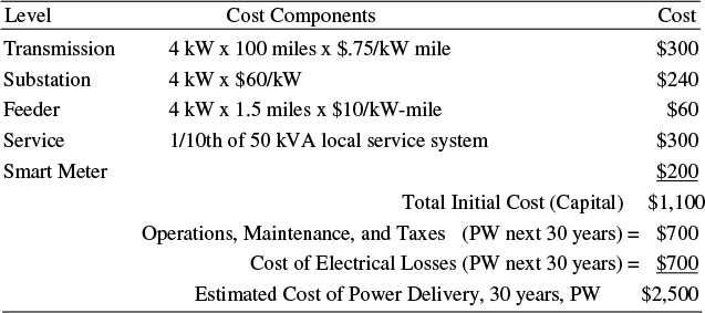
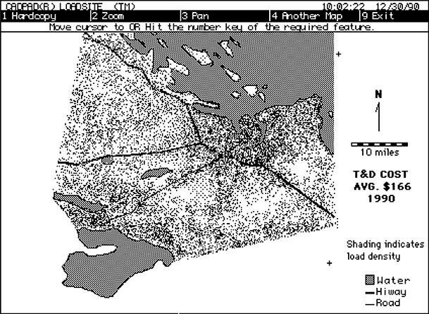
Figure 2.9 Cost of power delivery varies depending on location. Shown here are the annual capacity costs of delivery evaluated on a ten-acre basis throughout a coastal city of population 250,000. Cost varies from a low of $85/kW to a high of $270/kW.
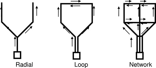
Figure 2.10 Simplified illustration of the concepts behind three types of power distribution configuration. Radial systems have only one electrical path from the substation to the consumer, loop systems have two, and networks have several. Arrows show most likely direction of electric flows.
A further attribute of most radial feeder system designs, but not an absolutely critical element, is the use of single-phase laterals. Throughout North America, most utilities use single- and two-phase laterals to deliver power over short distances, tapping off only one or two phases of the primary feeder. This minimizes the amount of wire that needs to be strung for the short segment required to get the power in the general vicinity of a dozen or so consumers. These laterals are also radial, but seldom, if ever, end in a switch (they just end). There are many utilities, particularly urban systems in Europe, Africa, and Asia that build every part of the radial distribution system, including laterals, with all three phases.
Each service transformer in these systems feeds power into a small radial system around it, basically a single electrical path from each service transformer to the consumers nearby.
Regardless of whether it uses single-phase laterals or not, the biggest advantages of the radial system configuration, in addition to its lower cost, is the simplicity of analysis and predictability of performance. Because there is only one path between each consumer and the substation, the direction of power flow is absolutely certain. Equally important, the load on any element of the system can be determined in the most straightforward manner - by simply adding up the entire consumer loads “downstream” from that piece of equipment.
Before the advent of economical and widely available computer analysis, this alone was an overwhelming advantage, for it allowed simple, straightforward, “back of the envelope” design procedures to be applied to the distribution system with confidence that the resulting system would work well. The simplicity of analysis, and confidence that operating behavior is strictly predictable are still great advantages.
Because load and power flow direction are easy to establish, voltage profiles can be determined with a good degree of accuracy without resorting to exotic calculation methods. Capacity requirements can be ascertained exactly. Fault levels can be predicted with accuracy and protective devices - breaker-relays and fuses - can be coordinated in an absolutely assured manner, without resorting to network methods of analysis. Regulators and capacitors can be sized, located, and set using relatively simple procedures (simple compared to those required for similar applications to non-radial designs in which the power flow direction is not a given).
On the debit side, radial feeder systems are less reliable than loop or network systems because there is only one path between the substation and the consumer. Thus, if any element along this path fails, a loss of power delivery results. Generally, when such a failure occurs, a repair crew is dispatched to re-switch temporarily the radial pattern network, transferring the interrupted consumers onto another feeder, until the damaged element can be repaired. This minimizes the period of outage, but an outage still occurred because of the failure.
Despite this apparent flaw, radial distribution systems, if well designed and constructed, generally provide very high levels of reliability. For all but the most densely populated areas, or absolutely critical loads (hospitals, important municipal facilities, the utility's own control center) the additional cost of an inherently more reliable configuration (loop or network) cannot possibly be justified for the slight improvement that is gained over a well-designed radial system.
An alternative to purely radial feeder design is a loop system consisting of a distribution design with two paths between the power sources (substations, service transformers) and every consumer. Such systems are often called "European," because this configuration is the preferred design of many European utilities, as well as European electrical contractors when called upon to lay out a power distribution system anywhere in the world. Equipment is sized and each loop is designed so that service can be maintained regardless of where an open point might be on the loop. Because of this requirement, whether operated radially (with one open point in each loop), or with closed loops, the basic equipment capacity requirements of the loop feeder design do not change.
Some urban areas in Europe and Asia are fed by multiple hierarchical loop systems. A 100+kV sub-transmission loop routes power to several substations, out of which several loop feeders distribute power to service transformers, which each route powers through a long loop secondary.
In terms of complexity, a loop feeder system is only slightly more complicated than a radial system. Power usually flows out from both sides toward the middle, and in all cases can take only one of two routes. Voltage drop, sizing, and protection engineering are only slightly more complicated than for radial systems.
But if designed thus, and if the protection (relay-breakers and sectionalizers) is also built to proper design standards, the loop system is more reliable than radial systems. Service will not be interrupted to the majority of consumers whenever a segment is outaged, because there is no “downstream” portion of any loop.
The major disadvantage of loop systems is capacity and cost. A loop must be able to meet all power and voltage drop requirements when fed from only one end, not both. It needs extra capacity on each end, and the conductor must be large enough to handle the power and voltage drop needs of the entire feeder if fed from either end. This makes the loop system inherently more reliable than a radial system, but the larger conductor and extra capacity increase costs.
Distribution networks are the most complicated, the most reliable, and in very rare cases also the most economical method of distributing electric power. A network involves multiple paths between all points in the network. Power flow between any two points is usually split among several paths, and if a failure occurs it instantly and automatically re-routes itself.
Rarely does a distribution network involve primary voltage-level network design, in which all or most of the switches between feeders are closed so that the feeder system is connected between substations. This is seldom done because it proves very expensive and often will not work well.9 Instead, a "distribution network" almost always involves "interlaced" radial feeders and a network secondary system - a grid of electrically strong (i.e., larger than needed to feed consumers in the immediate area) conductor connecting all the consumers together at utilization voltage. Most distribution networks are underground simply because they are employed only in high-density areas, where overhead space is not available.
In this type of design, the secondary grid is fed from radial feeders through service transformers, basically the same way the secondary is fed in radial or loop systems. The feeders are radial, but laid out in an interlaced manner - none has a sole service area, but instead they overlap. The interlaced configuration means that alternate service transformers along any street or circuit path are fed from alternate feeders, as shown in Figure 2.11.
While segments from two feeders always run parallel in any part of the system, the same two feeders never overlap for all of their routing. The essence of the interlaced system (and a design difficulty in any practical plan) is to mix up feeders so that each feeder partially parallels a few other feeders. Thus, if the feeder fails, it spreads its load out over a few other feeders, overloading none severely (Figure 2.12).
9 The major reason is this puts feeder network paths in parallel with transmission between substations, which results in unacceptable loop and circular flows as well as large dynamic shifts in load on the distribution system.
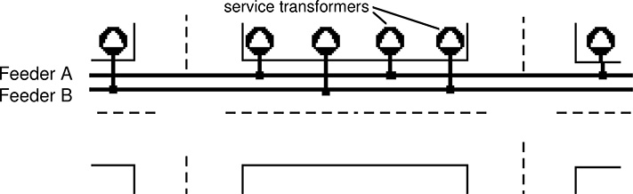
Figure 2.11 To obtain an interlacing factor of 2, two feeders are routed down each street, with alternating network transformers fed from each.
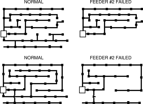
Figure 2.12 Top: a non-interlaced feeder system experiences the loss of one feeder, and all transformers in the lower right part of the system are lost - service is certain to be interrupted. Bottom: the same system interlaced. Loss of the feeder is a serious contingency, but can be withstood because the feeder losses are distributed in such a way that transformers still in service surround each transformer out of service.
At a minimum, distribution networks use an interlacing factor of two, meaning that two feeders overlap in any one region, each feeding every other service transformer. But such a system will fail when any two feeders are out of service. Interlacing factors as high as five (four overlapping feeders, each feeding every fourth
Networks have proven more expensive but more reliable than radial distribution systems. In urban applications where the load density is high, the electric facilities must be placed underground, and repairs and maintenance are difficult because of traffic and congestion, networks may cost only a little more to build and maintain that other types of underground systems. The best network systems can tolerate the loss of any three feeders (the other two in any area picking up the remaining load, although often very overloaded) without any interruption of consumer service. Networks require only a little more conductor capacity than a loop system. The loop configuration required “double capacity” everywhere to provide increased reliability.
Networks have two disadvantages. First, they are much more complicated, than other forms of distribution, and thus much more difficult to analyze and more expensive to operate. There is no “downstream” side to each unit as in a radial or loop system, so that the load seen by any unit of equipment cannot be obtained by merely adding up consumers on one side of it, nor can the direction of power flow through it be assumed. Loadings and power flow, fault currents and protection must be determined by network techniques such as those used by transmission planners. However, even more sophisticated calculation methods than those applied to transmission may be required, because a large distribution network can consist of 50,000 nodes or more - the size of the very largest transmission-level power pool. Distribution network load flows are often more difficult to solve than transmission systems because the range of impedance in the modeled circuits is an order of magnitude wider.
The second disadvantage distributed and distribution networks can have in comparison to other types of distribution designs is in system protection and in the field force safety procedures. Networks can – in fact usually do – have extremely high fault duties in the vaults and manholes where electrical equipment is located. The authors have seen fault levels as high as 160,000 amps on the low side of distributed network transformers in large downtown networks. Proper use of protective suits and gear, and good work practices, can mitigate any hazard to workers in such vaults, but these prudent precautions cost money and slow the pace of maintenance and service compared to what can be done on systems with lower fault levels. This cost issue has caused more than one utility to decide to convert older distributed networks to another type of distribution system, such as primary select radial switching.
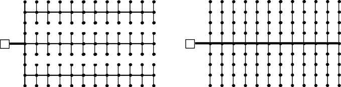
Figure 2.13 Two ways to route a radial feeder to 108 service transformers. Left, a "multi-branch" configuration. Right, a "large trunk" design.
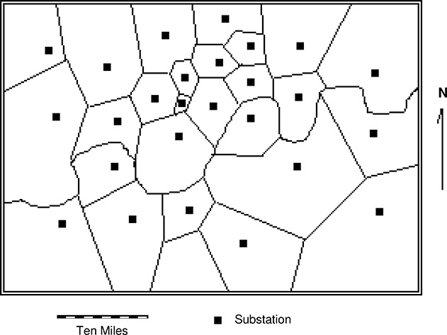
Figure 2.14 A power system is divided by substation service boundaries into a set of substation service areas, as shown.
Large-Trunk vs. Multi-Branch Feeder Layout
Figure 2.13 illustrates the basic concept behind two different ways to approach the layout of a radial distribution system. Each has advantages and disadvantages with respect to the other in certain situations, and neither is superior to the other in terms of reliability, cost, ease of protection, and service quality. Either can be engineered to work in nearly any situation. Most planning utilities have an institutionalized preference for one or the other. Beyond showing that there are significantly different ways to lay out a distribution system, this brings to light an important point about distribution design: major differences in standards exist among electric utilities, as a result of which comparison of statistics or practice from one to the other is often not valid. Feeder layout types and practices are discussed in much greater detail in the Power Distribution Planning Reference Book.
Service Areas
As mentioned earlier, in most power systems, each substation is usually the sole provider of electrical service to the region around it - its service area. Similarly, feeders and distribution networks also have distinct service areas. Usually, the service area for a substation, feeder, or other unit of equipment is the immediate area surrounding it, and usually these service areas are contiguous (i.e. not broken into several parts) and exclusive - no other similar distribution unit serves any of the load in an area. As an example, Figure 2.14 shows a map of substation service areas for a rectangular portion of a power system. Each distribution substation exclusively serves all consumers in the area containing it.
Cumulatively, the simultaneous peak demand of all customers in its service area defines the maximum power the substation must serve. Within a power system, each individual part, such as a substation or service transformer, will see its peak load at whatever time and in whatever season the consumers in its service area generate their cumulative peak demand. One result of this is that the peak loads for different substations often occur at different seasons of the year or hours of the day. But whenever the peak occurs, it defines the maximum power the unit is required to deliver. Peak demand is one of the most important criteria in designing and planning distribution systems. Usually it defines the required equipment capacity.
Dynamic Service Area Planning
By making switching changes in the distribution system, it is possible to expand or shrink a substation or feeder’s service area significantly, increasing or decreasing its net load. This is an important element of T&D planning, as shown in Figure 2.15, which illustrates a very typical T&D expansion situation. Two neighboring substations, A and B, each have a peak load near the upper limit of their reliable load-handling range. Load is growing slowly throughout the system, so that in each substation annual peak load is increasing at about 1 MW per year. Under present conditions, both will need to be upgraded soon. Approved transformer types, required to add capacity to each, are available only in 25 MVA increments, costing $500,000 each. Both substations do not need to be reinforced. A new 25 MVA transformer and associated equipment are added to substation A, increasing its ability to handle a peak load by about 20 MVA. Ten MW of substation B’s service area is then transferred to substation A. The result is that each substation has 10 MW of margin for continued load growth - further additions are not needed for 10 years.
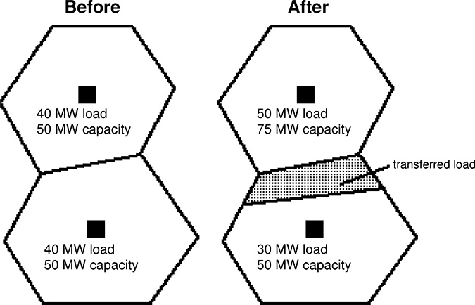
Figure 2.15 Load in both substations is growing at about 1 MW per year. Each substation has sufficient capacity to handle present load within contingency criteria (a 25% margin above peak) but nothing more. By transferring load as shown above, only one substation has to be reinforced with an additional (25 MVA) capacity, yet both end up with sufficient margin for another ten years’ growth. Service area shifts keep expansion costs down in spite of the fact that equipment like transformers are available only in large, discrete sizes.
This type of planned variation in service areas is a major tool used to keep T&D expansion costs low, a key element in building a reliable, economical schedule of expansion. Optimization of this particular aspect of planning can be a challenge, not because of any inherent difficulty in analysis, but simply because there are so many parts of the system and constraints to track at one time. This is one reason for the high degree of computerization in distribution planning at many utilities. Balancing the myriad requirements of many substations and their design and operating constraints is an ideal problem for numerical optimization techniques.
The Systems Approach
One complication in determining the most economical equipment for a power system is that its various levels - transmission, substation, and distribution - are interconnected, with the distribution in turn, connected to the consumers and hence a function of the local load density. The best size and equipment type at each level of the system is a function of the types of equipment selected for the other levels of the system and the load density. In general, the equipment is so interconnected that it is impossible to evaluate any one aspect of design without taking all others into account.
Consider the question of substation spacing - determining how far apart substations should be, on average for best utilization and economy. Within any service territory, if substations are located farther apart, there will be fewer of them, saving the utility the cost of buying and preparing some substation sites, as well as reducing the cost of building a large number of substations.
Thus, overall substation cost is a function of spacing, but how it varies depends on land and equipment costs, which must be balanced carefully. With fewer substations however, each substation must serve a larger area of the system. Hence, each substation will have a larger load and thus require a larger capacity, meaning it must have more or larger transformers.
The larger substations will also require a larger amount of power to be brought to each one, which generally calls for a higher sub-transmission voltage. Yet there will be fewer sub-transmission lines required because there are fewer substations to which power must be delivered. All three aspects of layout are related - greater substation spacing calls for larger substations with bigger transformers, and a higher transmission voltage, but fewer lines are needed - and all three create better economies of scale as spacing is increased. Thus, transmission costs generally drop as substation spacing is increased.
Nevertheless, there is a limit to this economy. The distribution feeder system is required to distribute each substation's power through its service area, moving power out to the boundary between each substation’s service area and that of its neighbors. Moving substations farther apart means that the distribution system must move power, on average, a greater distance. Distributing power over these longer distances requires longer and more heavily loaded feeders. This situation increases voltage drop and can produce higher losses, all of which can increase cost considerably. Employing a higher distribution voltage (such as 23.9 kV instead of 13.8 kV) improves performance and economy, but it costs more to distribute power from a few larger substations farther apart, than to distribute it from many smaller substations close together. Feeder costs go up rapidly as substation spacing is increased.
The major point of this section is that all four of the above aspects of system design are interconnected - 1) substation spacing in the system, 2) size and number of substations, 3) transmission voltage and design and, 4) distribution feeder voltage and design. One of these factors cannot be optimized without close evaluation of its interrelationship with the other three. Therefore, determining the most cost-effective design guideline involves evaluating the transmission-substation-feeder system design as a whole against the load pattern, and selecting the best combination of transmission voltage, substation transformer sizes, substation spacing, and feeder system voltage and layout.
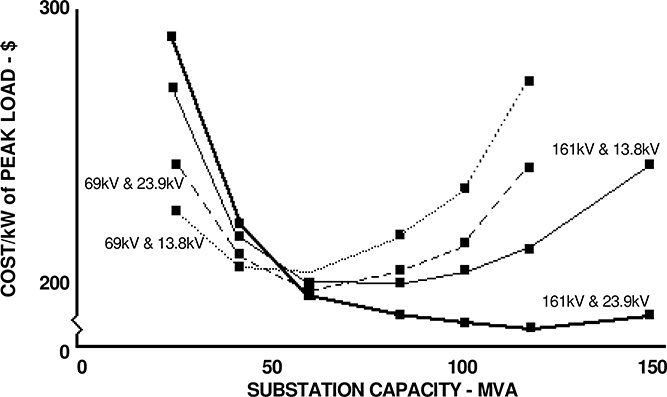
Figure 2.16 Overall cost of a T&D system depends on the balanced design of the sub-transmission, substation, and feeder level, as described in the text. Cost can vary by significant margins depending on how well performance and economy at various levels of the system are coordinated.
This economic equipment sizing and layout determination is based on achieving a balance between two conflicting cost relationships:
1. Higher voltage equipment is nearly always more economical on a per-MW basis.
2. Higher voltage equipment is available only in large sizes (lots of MW).
In cases where the local area demands are modest, higher voltage equipment may be more expensive simply because the minimum size is far above what is required - the utility has to buy more than it needs. How these two cost relationships play against one another depends on the load and the distances over which power must be delivered. Other factors to be considered are those unique to each power system, such as the voltages at which power is delivered from the regional power pool, and whether the system is underground or overhead.
Figure 2.16 illustrates the difference that careful coordination of system design between levels of the power system can have in lowering overall cost. Shown are the overall costs from various combinations of a T&D system layout for a large metropolitan utility in the eastern United States. Each line connects a set of cost computations for a system built with the same transmission and distribution voltages (e.g., 161 kV transmission and 13.8 kV distribution) but varying in substation sizes (and hence, implicitly, their spacing).
In all cases, the utility had determined it would build each substation with two equally sized transformers (for reliability), with none over 75 MVA (larger transformers are too difficult to move along normal roads and streets, even on special trailers). Either 161 kV or 69 kV could be used as sub-transmission, either
23.9 kV or 13.8 kV could be used as distribution voltage. Any size transformer, from 15 MVA to 75 MVA could be used, meaning the substation could vary from 30 MVA to 150 MVA in size. (Peak load of such substations can normally be up to 75% of capacity, for a peak load of from 23 to 100 MW.)Substation spacing itself is implicit and not shown. Given the requirement to cover the system, determining transmission voltage, distribution, and substation size defines the system design guidelines entirely.
Overall, the ultimate and lowest cost T&D system guidelines are to build 120 MVA substations (two 60 MVA transformers) fed by 161 kV sub-transmission and distributing power at 23.9 kV. This has a levelized cost (as computed for this utility) of about $179/kW. In this particular case, a high distribution voltage is perhaps the most important key to good economy - if 13.8 kV is used instead of
23.9 kV as the primary voltage, minimum achievable cost rises to $193/kW.
The very worst design choices plotted in Figure 2.16, from an economic standpoint, would be to build 25 MVA substations fed by 161 kV sub-transmission and feeding power to 23.9 kV feeders ($292/kW). This would require many small substations, each below the effective size of both the transmission and distribution voltages, and lead to high costs. Overall, 161 kV and 23.9 kV are the correct choices for economy, but only if used in conjunction with a few, large substations. If substations are to be 25 MVA, then 69 kV and
13.8 kV do a much more economical job ($228/kW), but still don't achieve anything like the optimum value. The point: Achieving economy in power delivery involves coordinating the interactions, performance, and economies of the multiple system levels. Chapters 11 and 12 discuss the issues of and techniques for such coordinated multi-level planning.
2.8 SMART GRID
Smart Grid refers to power systems that use sensors, digital and analog electronic control, and data communications among equipment and between the system and utility control centers, to enhance the capabilities and performance of the power system. Although the term “grid” typically refers to only the high-voltage (wholesale transmission) portion of a power system, the term “smart grid” is widely used to refer to any and all parts of a power system that employs such technology. Beyond the inclusion of a great deal of “high technology” and data communication into the equipment and system, a key element of a Smart Grid is that the design of the power system itself, and way it is operated, are also changed in recognition and to take full advantage of the capabilities that the smart equipment provides.
For example, the traditional design for primary distribution in North America is to lay out circuits in a radial configuration and to arrange sectionalization (where and how fuses opened if there were problems) in a cascading sequence up and down the circuit. As was discussed in Section 2.7, the chief advantage of this approach is simplicity, of design, protection coordination, and operation, to a degree that fit the needs of the period during which the industry settled on this approach (first quarter of the 20th century). Circuits can be successfully designed and equipment properly specified with a minimum of information and, quite literally, on the back of the envelope calculations. 10 The system is straightforward to operate, dispatch, and refer in a safe manner with only maps as databases and common sense procedures used to assure safety. The industry stuck with radial distribution systems throughout the 20th century and into the 21st because they provided satisfactory performance for the time and no change was needed. Considerable improvement in every and all aspects of a power distribution system’s performance can be achieved if a more complicated basic design approach is used as compared to simple radial configurations. System cost, customer service reliability, voltage stability, power quality, electric losses, and safety can all be improved at the same time. The price paid for the simplicity of early radial distribution systems is a substantial margin in equipment and system capability that is often there but unused. In the early 20th century, this margin covered all the unknowns due to engineers and operators not having comprehensive load and system metering data at their fingertips, and for the approximations used in back-of-the-envelope calculations, so that circuits designed with linear models of non-linear processes would still work well.
10 This is not to say one cannot do a somewhat better job at assuring good performance and lowered cost using the greater data gathered by modern IT systems and the computerized tools in wide use today. However, with only a pencil and paper, and estimates of number of customers and peak load/customers, a competent engineer can layout a radial distribution system so it will work satisfactorily when all equipment is functioning as intended and fail safe when something goes wrong. In a period when the most advanced tools available to power engineers were a slide rule and a book of logarithms, this was a necessity.
A system designed without that margin can be cheaper – perhaps up to 15% lower in overall cost – and more reliable with better quality of service. But engineers will need much more data in order to plan and engineer it. Modern smart data acquisition systems can gather this data, and modern Enterprise IT systems can provide it to the engineers in a way they can efficiently use it. Further, system operators will find the system a challenge to operate compared to the traditional radial system. It will require that they constantly adjust equipment settings in response to changes in load and system conditions, and that from time to time they recognize the system is in a different operating mode and that they have to re-orient some of its basic scheduling rules and priorities in order to assure that it “fails safe” should something go wrong.
All of this can be accommodated, usually in a completely automatic way, by the proper use of smart grid equipment and designs. The distribution system is no longer entirely radial in configuration or operation. It is deliberately designed so that it will have to change its configuration (switching) and equipment settings (voltage tap levels and capacitor switching) in order to function well throughout the course of a year or even perhaps a single day. Automatic equipment can do that. Protection and fail safe capability require that one unit of equipment “know” the status and loading of others nearby: data communication can provide this.
The net result is that a smart distribution system has better performance in every category than a traditional system, including the performance category cost. There is a price to pay, however. Smart systems are much more complex from nearly every standpoint, and require advanced design tools and planners, engineers and operators of exceptional skill and training to plan, design, and operate them.
2.9 CONCLUSION
A transmission and distribution system moves power from a utility’s power production and purchase points to its consumers. The T&D system’s mission of delivering power to the consumers means that it must be composed of equipment spread throughout the service territory and arranged locally so that capacity is always in proportion to local electrical demand. The facilities need to be in each neighborhood, sized and configured both to fit well into the whole and to serve the local needs. In the authors’ opinion, engineering a system to meet this challenge is seldom easy, but engineering a system to do so at the minimum possible cost is always extremely challenging.
A T&D system is composed of several interconnected, hierarchical levels, each of which is required for completion of the power delivery task. These levels are:
1. Transmission
2. Sub-transmission
3. Substation
4. Feeder
5. Secondary
6. Consumer
To a certain extent, the burden of power delivery, and costs, can be shifted from one level to another through changes in the specifications of equipment, layout standards, and design of the various levels. For example, costs can be pared at the substation level by using fewer, larger substations. This means, feeders in each substation area will have to carry power farther, and perhaps carry more power per feeder as well, increasing feeder costs. Low overall design cost is achieved by balancing these factors.
The performance and economy and thus the design of a power system are dominated by a number of constraints due to physical laws, and further shaped by a number of practical considerations with regard to equipment, layout, and operating requirements. The more important of these are:
1. The T&D System Must Cover Ground. This is the rule about T&D -ultimately the electric system must “run a wire” to every consumer. A significant portion of the cost of a distribution system is due to this requirement alone, independent of the amount of peak load or energy supplied.
2. Interconnectivity of Levels. The sub-transmission/substation-feeder triad comprises a highly interconnected system with the electrical and economic performance at one level heavily dependent on design, siting, and other decisions at another level. To a certain extent the T&D system must be planned and designed as a whole - its parts cannot be viewed in isolation.
3. Discrete Equipment Sizes. In many cases equipment is available only in certain discrete sizes. For example, 69 kV/12.47kV transformers may be available only in 5, 10, 20, and 22 MVA sizes. Usually, there is a large economy of scale - the installed cost of a 20 MVA unit being considerably less than two times that for a 10 MVA unit.
4. Dynamic Service Area Assignment is a Powerful Planning Tool. Maximization of equipment utilization and minimization of cost per unit of capacity can be obtained despite the fact that capacity upgrades can be built only in one of several discrete sizes. To accomplish this the planner changes the boundaries of the service area during the planning process. When reinforced with new capacity additions, a substation might pick up load from surrounding substations, effectively spreading the capacity addition among several substations.
5. Losses Cost Can Be Significant. In some cases, the present worth of future losses on a line or heavily loaded transformer can exceed its total capital cost. In most cases, this does not happen. But in most cases, the present worth of losses is greater than the difference in cost between most of the choices available to the planner. This means loss is a major factor to be considered in achieving overall least-cost design.
6. Cost to Upgrade is Greater than the Cost to Build. For example, one mile of a 12.47 kV, three-phase feeder using a 600 MCM conductor (15 MW thermal capacity) might cost $150,000 to build, and one mile of 9 MW feeder (336 MCM conductor) might cost only $110,000. But the cost to upgrade the 336 MCM feeder to 600 MCM wire size at a later date would be about $130,000, for a cumulative total of $240,000. Therefore, one aspect of minimizing cost is to determine size for equipment not on the basis of immediate need, but by assessing the eventual need and determining whether the present worth of the eventual savings warrants the investment in larger size now.
7. Coincidence of Peaks. Not all consumer loads occur at the same time. This has a number of effects. First, peak load in different parts of the system may occur at different times. Second, the system peak load will always be less than the sum of the peak loads at any one level of the system. For example, in more power systems the sum of all substation peak loads usually exceeds system total peak by 3% to 8%. Diversity of peak loads means that considerable attention must be paid to the pattern and timing of electric load if equipment needs (and consequently costs) are to be minimized.
8. Reliability is Obtained through Contingency Margin. Traditionally, T&D reliability in a static system (one without automation, and hence incapable of recognizing and reacting to equipment outages and other contingencies by re-configuring and/or re-calibrating equipment) is assured by adding an emergency, or contingency margin throughout the system. At the T&D level this means that an average of 20% to 50% additional capacity is included in most equipment, so that it can pick up additional load if neighboring equipment fails or is overloaded.
A Complicated System
In conclusion, a power T&D system provides the delivery of an electric utility’s product. It must deliver that product to every consumer’s site, with high reliability and in ready-to-use form. While composed of equipment that is individually straightforward, most T&D systems are quite complex due to the interactions of thousands, even millions, of interconnected elements. Achieving economy and reliability means carefully balancing a myriad of mutual interactions with conflicting cost tradeoffs.
REFERENCES AND BIBLIOGRAPHY
R.E. Brown, Electric Power Distribution Reliability – Second Edition, CRC Press, Boca Raton, 2009.
R.E. Brown, Business Essentials for Utility Engineers, CRC Press, Boca Raton, 2010.
J. J. Burke, Power Distribution Engineering – Fundamentals and Applications, Marcel Dekker, New York, 1994.
M. V. Engel et al., editors, Tutorial on Distribution Planning, IEEE Course Text EHO 361-6-PWR, Institute of Electrical and Electronics Engineers, Hoes Lane, NJ, 1992.
A. C. Monteith and C. F. Wagner, Electrical Transmission and Distribution Reference Book, Westinghouse Electric Company, Pittsburgh, PA, 1964.
H. L. Willis, Power Distribution Planning Reference Book – Second Edition, Marcel Dekker, New York, 1997.
H. L. Willis and W. G. Scott, Distributed Power Generation – Planning and Evaluation, Marcel Dekker, New York, 2000.