
3
Molecular Imaging True Color Spectroscopic (METRiCS) Optical Coherence Tomography
Adam Wax and Francisco E. Robles
CONTENTS
3.2 Dual-Window Signal Processing
3.3 Fourier Domain Low Coherence Interferometry: Analysis of Scattering Features
3.4 Molecular Imaging True Color Spectroscopic (METRiCS) OCT: Analysis of Absorption Features
3.1 Introduction
Optical coherence tomography (OCT) is a cross-sectional high-resolution optical imaging modality that operates under the principles of low coherence interferometry (LCI) to enable optical sectioning, or depth resolution, within a biological sample [1]. OCT has been particularly successful for application in ophthalmology where the optical transparency of the eye, especially for wavelengths in the near-infrared region of the spectrum, allows high-resolution visualization of retinal layers for diagnosing diseases and assisting in surgeries [2]. Although originally implemented in a time domain approach where mechanical scanning of a reference mirror in an interferometry scheme enabled measurement of depth resolved reflection profiles (A-scans), recent technological advances in OCT have led to the dominance of frequency domain (FD-) OCT due to its improved acquisition speed [3] and sensitivity [4]. As the name suggests, FD-OCT measures interferometric data as a function of frequency and a Fourier transform is used to produce the A-scan, typically with an axial resolution of a few micrometers and imaging depths of 1–2 mm. To implement tomographic images, multiple A-scans are obtained using transverse scanning or a parallel acquisition scheme.
Figure 3.1a illustrates a typical FD-OCT system, where a source with a wide bandwidth, S(λ), is split into a sample field, ES, and reference field, ER. The sample field ES interacts with a sample while the reference field ER is reflected off a reference mirror. In this example, light remitted from three different locations in the sample (m = 1, 2, and 3) is mixed with the reference field and detected using a spectrometer. Because the interferometric signal is recorded as a function of wavelength (i.e., in the frequency domain), it must be resampled to a linear wavenumber vector, k = λ/2π (Figure 3.1b), to enable recovery of the A-scan (Figure 3.1c) via a fast Fourier transform (FFT).
Although the majority of clinical OCT imaging instruments measure structure by the intensity of returned light, various extensions of OCT have allowed for other parameters to be assessed: of particular relevance here is spectroscopic OCT (SOCT), which provides additional information by measuring the spatially dependent spectrum of light.
SOCT supplements the high-resolution imaging capabilities of OCT with the rich source of information available via optical spectroscopy. In this approach, the wide spectral bandwidth of the low coherence light sources required for depth sectioning is exploited to obtain spectral information. Processing of SOCT signals typically uses a short-time Fourier transform (STFT) or continuous wavelet transform (CWT) to identify the spatially varying, spectral properties of samples. Figure 3.2 illustrates STFT processing of SOCT signals. In this example, light returned from the ideal sample, simulated in Figure 3.1, undergoes attenuation, reducing the spectral intensity returned from deeper scatterers at certain wavelengths (Figure 3.2a). An STFT entails using a window that is swept across the full bandwidth with an FFT computed at each step (Figure 3.2b). The output is a time frequency distribution (TFD) map that describes the spectrum returned by each sample point. A significant limitation of the STFT is that there is a trade-off associated with the width of the window used in this process. If the window is chosen to be large in spectrum, then the TFD contains high spatial resolution, but suffers from poor spectral resolution and vice versa.
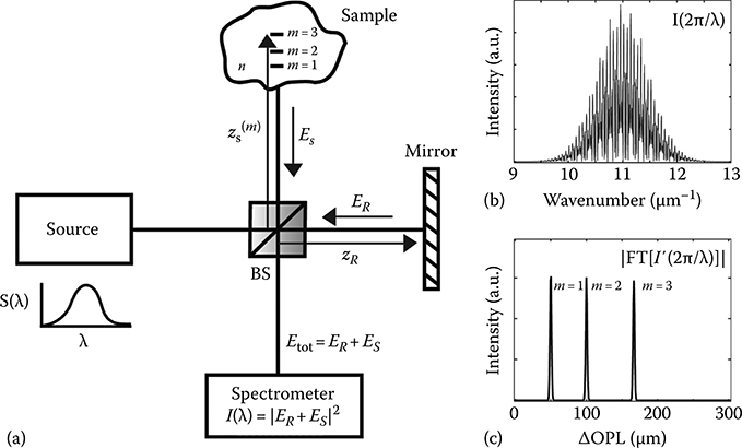
FIGURE 3.1
(a) Schematic of FD-OCT system. (b) Interferogram resampled into a linear wavenumber vector. (c) A-scan: absolute value of the Fourier transform of (b) after back ground subtraction. See text for details. (Taken from Robles, F.E., Light scattering and absorption spectroscopy in three dimensions using quantitative low coherence interferometry for biomedical applications, PhD thesis in Medical Physics, Duke University, Durham, NC, 2011.)

FIGURE 3.2
(a) Relative wavenumber (or wavelength) intensity returning from three simulated scatterers, as shown in Figure 3.1. (b) SOCT processing using STFT. (c) Resulting time frequency distribution (TFD). (Taken from Robles, F.E., Light scattering and absorption spectroscopy in three dimensions using quantitative low coherence interferometry for biomedical applications, PhD thesis in Medical Physics, Duke University, Durham, NC, 2011.)
SOCT was first introduced by Morgner et al., and was used only to assess the center-of-mass of depth-resolved spectra to provide an additional mechanism of contrast [6]. However, more recent studies have explored using the full spectrum to obtain detailed functional information. For example, Faber et al. [7] and Yi et al. [8] have used SOCT to quantitatively measure the absorption coefficient of Hb. SOCT also can be used to detect the presence of exogenous contrast agents that tag specific cell receptors or trace functional mechanisms. This approach has been explored by Cang et al. who used SOCT to detect plasmonic gold nanocages in tissue phantoms [9] and by Oldenberg et al. using SOCT to detect nano rods in ex vivo human breast carcinoma [10].
To date, SOCT has not been widely applied to in vivo imaging or for preclinical studies of disease mechanisms. One view is that progress in its development has been limited by the trade-off between spatial and spectral resolution, as previously mentioned. While this trade-off is inherent in the STFT, it is not necessarily present for other methods that reconstruct TFDs; for example, bilinear distributions can avoid this limitation, although they typically have their own unique trade-offs. The widespread use of the near-infrared spectrum in OCT has also been a limiting factor in biomedical studies using SOCT, especially since biological absorbers such as hemoglo-bin have relatively low absorption in this range resulting in low confidence intervals [11].
In this chapter, we describe advancement of SOCT to enable depth resolved spectroscopy. By using a novel dual window processing method [12], the trade-off between depth and spectral resolution is effectively removed, enabling high resolution in both domains. We have advanced the DW SOCT method in two directions: Fourier domain low coherence interferometry (fLCI) for employing spectral information for analyzing scattering properties and molecular contrast true color SOCT (METRiCS OCT) for using the absorption properties of samples for true color display and to obtain functional information. The remainder of this chapter includes an overview of the DW method, discussion of its application to analyzing scattering, specifically for early cancer diagnosis, and then demonstration of its utility for analysis of absorption properties.
3.2 Dual-Window Signal Processing
Depth resolved spectroscopic information may be obtained from interferometric data to obtain functional information of a sample. As discussed earlier, a short-time Fourier transform (STFT) is typically used to access this information. This process uses a mathematical window to isolate information from a particular frequency range. When the windowed data are Fourier transformed to yield a depth resolved reflection profile, some depth resolution is lost due to the reduction of frequencies contributing to the signal. However, by sweeping the window across the full bandwidth of the source, a depth resolved reflection profile is obtained at each step, providing a map of the spectral content confined within a spatial (or depth) region (see Figures 3.2 and 3.3). The process produces a time–frequency distribution (TFD) of the signal; however, TFDs obtained using a single STFT are limited due to the inherent trade-off between the resulting spectral and the depth resolution. In order to produce distributions with high resolution in both dimensions, we have developed the dual window (DW) processing method.
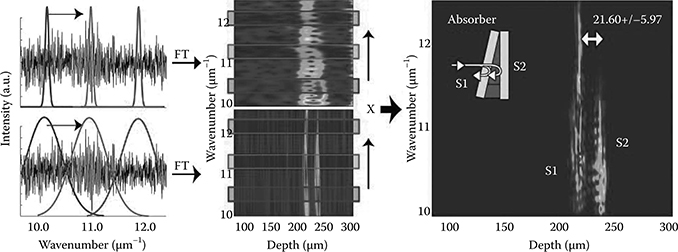
FIGURE 3.3
Procedure for calculating the DW TFD. The interferometric signal is generated from an absorbing phantom with two scattering surfaces, S1 and S2. (Adapted from Robles, F. et al., Opt. Express, 17(8), 6799, 2009.)
The DW method is based on calculating two separate STFTs and then multiplying the results. The first STFT uses a broad spectral Gaussian window to obtain high depth resolution, while the second STFT uses a narrow spectral window to generate high spectroscopic resolution. Thus, the resulting DW TFD simultaneously achieves high resolution in both dimensions. Mathematically, this can be described as
where ES, ER are the sample and reference fields, with the caveat that ER is assumed to vary slowly with respect to wavenumber. <…> denotes an ensemble average, ΔOPL is the optical path length difference between the sample and the reference arms, z is the axial distance, and w1 and w2 are the widths (standard deviation of the Gaussian distribution) of the two windows. Figure 3.3 illustrates the procedure for computing the DW TFD for a signal generated by an absorbing phantom with two scattering surfaces, S1 and S2.
From the DW TFD, one can observe that the two scattering surfaces are clearly spatially resolved, and that the spectrum from S2 exhibits absorption with a loss of intensity at specific wavenumbers. To assess the fidelity of the spectral information, Figure 3.4a and b shows the spectrum from the light returned from the two coverglass surfaces, S1 and S2, respectively. Here, we note that the spectral resolution of the STFT and the DW are comparable to that of the ideal case (obtained by a transmission measurement). However, the time marginals (TFD integrated with respect to wavenumber), shown in Figure 3.4c, demonstrate the superior depth resolution of the DW method compared to that of an optimized STFT. The spatial resolution of the STFT can be improved by choosing a wider spectral window; however, this process would degrade the spectral resolution.
The depth resolved spectra from the DW TFD in Figure 3.4 also contain high-frequency oscillations. These are termed local oscillations and can be analyzed to reveal structural information about the sample. By taking a Fourier transform of these oscillations (e.g., blue line in Figure 3.4a), a correlation function is produced (Figure 3.4d), which contains a clear peak at a correlation distance of 21.60 ± 0.57 μm. This distance corresponds to the spacing between the two scattering surfaces and can be compared to the distance obtained by imaging, 21.6 ± 5.97 μm (see Figures 3.3 or 3.4c). By analyzing the periodicity of the local oscillations, the scattering structures in the sample can be precisely measured. This mechanism is exploited in fLCI to recover information about the cell nuclear diameter in tissue [12]. A more rigorous mathematical description on the origin of the local oscillations can be found in Reference [12].

FIGURE 3.4
Depth resolved spectra from S1 (a) and S2 (b). (c) Time marginals. (d) Correlation function calculated by the Fourier transform of the DW depth resolved spectra from S1 (dotted line in (a)). The peak corresponds to the physical distance between S1 and S2. (Adapted from Robles, F. et al., Opt. Express, 17(8), 6799, 2009.)
3.3 Fourier Domain Low Coherence Interferometry: Analysis of Scattering Features
The fLCI approach analyzes depth-dependent, high-frequency spectral oscillations (described earlier as local oscillations) to measure the size of dominant scatterers in tissue. Through several studies of in vitro cells and tissues, the fLCI measurement has been associated with the diameter of cell nuclei [13–15]. As Figure 3.5 illustrates, light scattered by cell nuclei contains two components—one originating from the front surface and the second arising from the back surface—which interact to produce periodic oscillations in the resultant local scattering spectrum. The frequency of the oscillations is proportional to the optical path length difference of the two scattered field components. An important feature of this analysis is that the local oscillations are specific to the individual scatterer, and thus high spatial and spectral resolution are required to observe them. A loss of resolution in either domain will result in a decrease in visibility of these fringes and prevent an effective analysis.

FIGURE 3.5
(a) Light is incident on cell nuclei of different sizes. (b) Localized spectra which exhibit local oscillations resulting from the induced temporal coherence of the light that is scattered from the front and back surface of the nuclei. The periodicity of the local oscillations is proportional to the size of the cell nuclei. (Adapted from Graf, R. et al., J. Biomed. Opt., 14, 064030, 2009.)
The first demonstration of the fLCI technique was accomplished using a scattering phantom consisting of dried polystyrene beads on a coverglass [17]. A subsequent study validated the ability of the approach to measure cell nuclei in vitro, confirmed via confocal microscopy [18]. The planar geometry of these samples provided two-dimensional surfaces, and thus STFT processing could be used since the loss of depth resolution was not relevant. However, the trade-off in resolution associated with STFTs precluded analysis of local oscillations in more complex, three-dimensional biological samples.
To validate the DW fLCI approach, an analysis of the scattering properties of a turbid sample containing different populations of scatterers is presented. The analysis consists of processing an OCT image with the DW method and then using fLCI and light scattering spectroscopy (LSS) to obtain structural information. LSS extracts the size of spherical scatterers by analyzing periodicity in the spectrum of singly scattered light [19]. The periodic spectral features correspond to the scattering cross section of spherical structures, and are well described by the Van de Hulst approximation [20]. These features are distinct from the local oscillations used in fLCI and exhibit lower-frequency spectral oscillations. Thus, fLCI and LSS measurements can be obtained simultaneously by looking at the high- and low-frequency components of the depth resolved spectra, respectively.
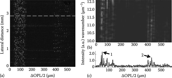
FIGURE 3.6
(a) Parallel frequency-domain OCT image of a two-layer phantom. The top layer (optical path length difference/2 [ΔOPL/2] ranging from 35 to 125 μm) contains 4.00 μm beads, while the bottom layer (400–550 μm) contains 6.98 μm beads. The dashed line corresponds to a single lateral line or A-scan (c) from which the DW TFD is generated (b). The spectra and correlation function of points 1 and 2 are analyzed later in Figure 3.7. (Adapted from Robles, F.E. and Wax, A., Opt. Lett., 35(3), 360, 2010.)
The sample for this experiment comprised two layers, each containing a different size of polystyrene microsphere (index of refraction nb = 1.59). The microspheres are suspended in a mixture of agar (2% by weight) and water (na = 1.35). The average size in the top layer is d = 4.00 ± 0.033 μm, and in the bottom layer d = 6.98 ± 0.055 μm. Figure 3.6a shows an OCT image of the phantom. The ability to obtain functional information from high-resolution OCT (and SOCT) images is a strength of the fLCI analysis since OCT inherently provides visual (or spatial) guidance for its functional analysis. The DW TFD is generated for each lateral line (or A-scan) of the OCT image with window sizes w1 = 0.0454 μm−1 (Δλ = 2.39 nm) for high spectral resolution and w2 = 0.6670 μm−1 (Δλ = 35.1nm) for high depth resolution. The resulting DW TFD, computed from the A-scan delineated by the dotted red line in Figure 3.6a, is shown in Figure 3.6b. Figure 3.6c is the corresponding A-scan [21].
The depth resolved DW spectra contain two components that relay structural information of the sample. The low-frequency component is analyzed using the Van de Hulst approximation [20], which describes the wavelength-dependent cross section of the scatterers (LSS method). The analysis is implemented by first low-pass filtering the DW spectral profile with a hard cutoff frequency of 3.5 μm (three cycles) and the resulting distribution is fit to the theoretical Van de Hulst model using a least-squares method. The low-pass filtered data used for fitting are shown in Figure 3.7a and b, which yield sizes of d1 = 3.97 μm and d2 = 6.91 μm for points 1 and 2 in Figure 3.7c, respectively, in good agreement with the known sizes: 4.00 ± 0.033 and 6.98 ± 0.055 μm [21].

FIGURE 3.7
(a) and (b) DW spectral profiles (solid lines) and low-pass filtered spectra (dotted curves) from points 1 to 2 in Figure 3.6c, respectively. Dashed lines are the theoretical scattering cross sections for 3.97 and 6.91 μm spherical scatterers for points 1 and 2, respectively. (c) and (d) Correlation function from points 1 and 2, with correlation distances (dc) of 4.25 and 6.87 μm, respectively. (e) Overlay of the fLCI measurements with the OCT image. (Adapted from Robles, F.E. and Wax, A., Opt. Lett., 35(3), 360, 2010.)
The second component of the depth resolved DW spectra, which consists of the local oscillations (high frequencies), is analyzed using fLCI. In this case, the local oscillations arise from induced temporal coherence effects between the fields scattered by the front and back surfaces of the microspheres. To compute structural information from this component, the spectral dependence is removed by subtracting the line of best fit from the LSS analysis described earlier. The residuals are then Fourier transformed to yield a correlation function [22], where the maximum peak indicates the round-trip optical path length (ΔOPL) through the scatterer. Figure 3.7c and d plot the correlation function for points 1 and 2, from Figure 3.6c, respectively. The correlation peaks for these points are located at dc = ΔOPL/(2nb) = 4.25 and 6.87 μm, in good agreement with both the LSS measurements and the known bead size in each layer [21].
The LSS and fLCI analyses were repeated for each A-scan and all points in the OCT image where the intensity exceeded the background level. Figure 3.7e shows the results by overlaying the fLCI measurements with the OCT image. The LSS map (not shown) yields similar results. In the top layer, the average scatterer size was 3.82 ± 0.67 and 3.68 ± 0.41 μm for the fLCI and LSS measurements, respectively (112 points). In the bottom layer, the average scatterer size was 6.55 ± 0.47 and 6.75 ± 0.42 μm for fLCI and LSS, respectively (113 points) [21].
The results of this phantom study show that the DW fLCI technique yields accurate and precise structural measurements based on spectral analysis of an OCT image. Previous efforts have only been able to recover limited details of scatterer structure, typically restricted to discriminating large and small objects. However, with the DW method, the resolution trade-off was avoided and enabled detection of local oscillations in tissue. With an eye toward early detection of cancerous lesions, Graf et al. applied fLCI to detect dysplasia using an ex vivo hamster cheek pouch carcinogenesis model. The results from this study yielded 100% sensitivity and 100% specificity, clearly demonstrating the potential of fLCI as a powerful diagnostic method [16].
To illustrate the utility of fLCI-based analysis of DW-processed OCT images, we present a study of ex vivo tissues drawn from the azoxymethane (AOM) rat carcinogenesis model, a well-characterized and established model for colon cancer research and drug development [23]. The model generates cancerous lesions in the colonic epithelium, arising from neoplastic aberrant crypt foci (ACF). In this study, we seek not only to use fLCI to identify the presence of ACF but also to identify systemic changes in the tissue characteristic of the field effect of carcinogensis. The phenomenon of the field effect describes observations that neoplastic development in one part of the colonic epithelium distorts nano- and microtissue morphology, as well as tissue function, along the entire organ. This phenomenon has been a subject of much interest since it indicates that adequate screening may be achieved by only probing certain (and more readily accessible) sections of the colon [24–26], thus suggesting a new avenue for less invasive screening for colorectal cancer (CRC). This study exploits the depth resolution of fLCI to compare the functional data of the ex vivo samples at three depths to identify changes indicative of early CRC development. The sensitivity of fLCI to the field effect is explored through measurements at two different longitudinal sections of the left colon.
All animal experimental protocols were approved by Institutional Animal Care and Use Committee of The Hamner Institute and Duke University. Forty F344 rats were randomized into groups of 10, with 30 receiving intraperitoneal (IP) injections of AOM >90% pure with a molar concentration of 13.4 M at a dose level of 15 mg/kg body weight, once per week, for two consecutive weeks (two doses per animal). The remaining 10 animals received saline by IP and served as the control group. At 4, 8, and 12 weeks after the completion of the dosing regimen, the animals (10 AOM-treated and 3 or 4 saline-treated rats per time point) were sacrificed by CO2 asphyxiation. The colon tissues were harvested, opened longitudinally, and washed with saline. The tissue was split into—four to five different segments, each with a length of 3–4 cm, where only the two most distal segments were analyzed: the distal left colon (LC) and proximal LC. After imaging, the tissue samples were fixed in formalin and stained with methylene blue in order to be scored based on the number of ACF.
Each sample was placed on a cover glass for examination with a parallel frequency domain (pfd) OCT system. This system enables acquisition of up to 400 OCT A-scans with a single camera exposure of 20–100 ms, depending on the choice of light source and sample. This system achieved a lateral resolution of 10 μm and an axial resolution of 1.1 μm. Since the fLCI analysis retrieves optical path length rather than physical thickness, an index of refraction of n = 1.395 is used to convert the optical path length to nucleus size [27]. For the generation of the DW TFDs, the window standard deviations used were w1 = 0.029 μm−1 and w2 = 0.804 μm−1, resulting in TFDs with an axial resolution of 3.45 μm and spectral resolution of 1.66 nm. The spatial information provided by the OCT images is used to co-register the spectroscopic information as a function of distance from the tissue surface, allowing for consistent analysis at specific tissue depths.
Once the depth segments are aligned, regions of interest are selected for analysis and the data are averaged for that region in order to provide sufficient fringe contrast of the local oscillations. In the lateral direction, 20 DW TFDs are averaged to yield 10 different lateral segments in each OCT image. In the axial direction, we calculate the spectral averages of 25 μm depth segments from three different sections: the first at the surface (surface section 0–25 μm), a second centered about 35 μm in depth (mid-section 22.5–47.5 μm), and a third centered about 50 μm in depth (low section 37.5–62.5 μm). Figure 3.8a illustrates a typical OCT image for an AOM-treated rat tissue sample, where the dotted line delineates a region of interest for the mid-depth section. The corresponding DW TFD (after alignment and averaging laterally) is shown in Figure 3.8b.
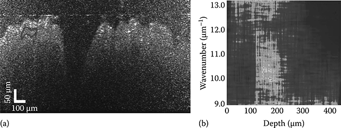
FIGURE 3.8
(a) pfdOCT image of an ex vivo rat colon sample. The line delineates an example region that is averaged across to determine the nuclear diameter. (b) DW TFD (after alignment and averaging laterally), of the laterally delineated region. (Adapted from Robles, F. et al., Biomed. Opt. Express, 1(2), 736, 2010.)
As described previously, the spectra from the averaged regions contain two components. The first component is the low-frequency oscillations, which may be analyzed with LSS; however, we have found that due to the lack of knowledge of the precise refractive index of the scatterer and the surrounding medium in tissue [29], the amount of useful information that can be extracted from this method is limited. Instead, the low-frequency oscillations here are isolated using a smoothing function and subtracted from the spectra. This process isolates the second component: the high-frequency components of the spectra arising from the local oscillations due to temporally coherent fields induced by the cell nuclei in the averaged region (fLCI method). Note that we assume that the cell nuclei contain a constant nuclear RI of nn = 1.395 for this analysis [27]. Figure 3.9a illustrates the depth resolved spectrum (blue solid line), along with the low-frequency component (dotted black line), for the average region shown in Figure 3.8a. Figure 3.9b shows the isolated local oscillations, and Figure 3.9c, is the corresponding correlation function with a peak at 7.88 μm corresponding to the average cell nuclear diameter in the region of analysis.
Statistical analysis of the data (using a two-sided student t-test) revealed that the most significant layer for diagnosis using fLCI was the mid-depth section, which includes the basal layer of the epithelium. This layer has been shown to be the most diagnostically useful for discriminating dysplastic tissues using light scattering analysis [30–34]. Based on this finding, data from the two tissue segments (proximal and distal left colon) were analyzed separately only for this depth section. The measured cell nuclear diameters and number of ACF are summarized in Figure 3.10. The data show that for all the time points, and for both segments, the measured nuclear diameters for the treated groups were significantly different from the control group (p-values < 10−4**). Furthermore, significant differences were observed for both segments after only 4 weeks post treatment. This measured increase in the nuclear diameter, however, remained relatively constant thereafter, with the exception of the last time point in the proximal LC. Here, the nuclear diameter increased dramatically from ∼6.0 to ∼7.2 μm. To investigate this effect further, Figure 3.10c plots the nuclear diameter as a function of the average number of ACF, which are neoplastic lesions in this model. For clarity, we also identify each point with its corresponding time period. Note that the formation of ACF was faster in the proximal LC compared to the distal LC, and that the plot shows a region of little nuclear morphological change after the initial formation of ACF. This plateau region is present in both sections and is initially independent of the number of ACF. However, once the number of ACF increased to the maximum value observed in this study (∼70), the measured increase of the nuclear diameter was specific to the region manifesting more advanced neoplastic development, in contrast to the ubiquitous and relatively constant cell nuclear diameter measurements of the plateau region [28]. These data suggest the presence of a systematic change in the tissue upon formation of neoplastic lesions in this model, suggesting that a field effect has been detected.

FIGURE 3.9
Average spectrum (solid line) from the delineated region in Figure 3.8, along with the low-frequency component (dotted line) (a). The low-frequency component is subtracted from the averaged spectrum to obtain the local oscillations (b). A Fourier transform yields a correlation function (c), where the peak corresponds to an average cell nuclear diameter of 7.88 μm in the region of analysis. (Taken from Robles, F. et al., Biomed. Opt. Express, 1(2), 736, 2010.)
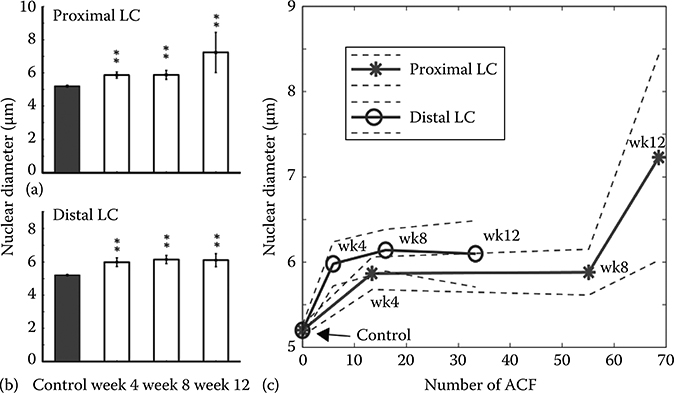
FIGURE 3.10
fLCI nuclear morphology measurements at different colon length segments. Highly statistical differences (p-value <10−4**) were observed between the control group and the treated groups for the proximal LC (a) and distal LC (b). (c) Plot of the measured cell nuclear diameter as a function of the number of ACF. For clarity, the time of measurement is noted next to each point (wk = week). (Taken from Robles, F. et al., Biomed. Opt. Express, 1(2), 736, 2010.)
This study showed that fLCI can be used to detect structural changes associated with neoplastic development, demonstrating the potential utility of the method. Further, the measured early nuclear morphological changes were observed in both tissue segments and independently of the number of ACF, indicating detection of a ubiquitous micromorphological change of the colonic epithelium due to the field effect. However, when neoplastic development became more advanced (demarcated by the high number of ACF), the nuclear diameter increase was specific to the affected region, supporting the claim that fLCI can identify specific regions where advanced neoplastic development has occurred. Both of these aspects point to a clinical utility of fLCI for detecting CRC development and identifying its location for targeting therapy.
3.4 Molecular Imaging True Color Spectroscopic (METRiCS) OCT: Analysis of Absorption Features
Molecular imaging holds a pivotal role in medicine, owing to its ability to provide invaluable insight into disease mechanisms at the molecular and cellular level. To this end, various techniques have been developed for molecular imaging, each with its own advantages and disadvantages [35–38]. For example, fluorescence imaging achieves micrometer-scale resolution, but has low penetration depths and is mostly limited to exogenous agents. In addition to enabling analysis of scattering features, the DW method can be applied to analyze depth-resolved, absorption spectral signatures of both endogenous and exogenous chromophores, enabling a novel form of SOCT capable of molecular imaging. The compelling feature of this new imaging modality is that simultaneous structural/morphological information is provided with micrometer-scale resolution in three dimensions
A key advance which has enabled METRiCS OCT is the use of a supercontin-uum laser light source in the pfdOCT system instead of the thermal light sources used in the experiments mentioned earlier. While both sources provide access to the visible region of the spectrum, the supercontinuum source avoids signal washout or loss of SNR due to coherent addition of multiple modes. With the thermal light source, this was mitigated by collimating the light incident on the sample, thereby separating these modes but resulting in a significant amount of light being discarded. Thus, imaging of biological samples could be achieved but the use of the thermal light source limited SNR to 89 dB [39], lower than most OCT systems (typically around 120 dB [4]). As an alternative source, super continuum laser sources offer a range that spans the visible spectrum yet offers a single spatial mode. This aspect enables focusing of the light to a diffraction limited point (or line) and allows for more photons to be collected, increasing SNR.
Figure 3.11 shows the pfd OCT system using the supercontinuum source (Fianium SC450–4, spectral range = 400−2000 nm, output power = 4 W, average power spectral density = 2 mW/nm). A series of filters are used to smooth the source spectrum across the detection bandwidth of 240 nm cen-tered at 575 nm. Note that the NIR components are not used for imaging here. This system yields an experimental axial resolution of 1.2 μm (limited by the source bandwidth and system dispersion) and penetration depth of 0.4 mm (limited by the spectral resolution of the spectrograph).

FIGURE 3.11
pfdOCT system with a super continuum laser source. The cylindrical lens delivers a line of illumination on the sample. The light path traced with the solid lines shaded in gray is in the y–z plane, where the light is focused onto the sample. The dotted line traces the light path in the x–z plane, where light is collimated onto the sample. (Taken from Robles, F.E., Light scattering and absorption spectroscopy in three dimensions using quantitative low coherence interferometry for biomedical applications, PhD thesis in Medical Physics, Duke University, Durham, NC, 2011.)
In this system, the light is focused in one dimension using a cylindrical lens, producing a line of illumination at the sample and reference mirror. Light returned from the sample is mixed with the reference field at the beamsplitter, and imaged onto the entrance slit of the imaging spectrograph. The lateral resolution is 6 μm, achieved by setting the focal lengths of L3 and L4 to 100 mm and L5 to 300 mm. Here, the use of relatively long focal length lenses minimizes the effect of chromatic aberrations.
For biomedicine, molecular imaging focuses on tissue blood content and oxygen levels, which are instrumental in diagnosing diseases. To obtain this information, METRiCS OCT takes advantage of the ability to measure depth resolved spectra to analyze the very distinct absorption features of oxygenated (oxy-) and deoxygenated (deoxy-) Hb. To illustrate how absorbing signatures may be quantified with SOCT, we consider an (S)OCT signal from one scatterer or reflector:
where IR = |ER|2 is the reference field intensity, IS = |ES|2 is the sample field intensity, and d is the round trip optical path length difference between the signal and the reference fields. In the case of a strongly absorbing sample, where scattering does not influence the spectra significantly, the modulation of the source field intensity may be described by S′(λ,zS(1)) = S(λ) · exp(−2μa(λ) · L), where μa(λ) is the absorption coefficient and L = d/(2n) is the distance from the surface of the absorbing sample to the scattering/reflecting point. Thus, the sample field intensity may be described as IS = R S(λ) · exp(−2μa(λ) · L), where R is the reflectance of the sample. Lastly, consider that that reference field intensity is equivalent to that of the source field, IR = S(λ), such that the OCT signal can be described as
where r is the reflectivity of the sample, r = √R. Note that the intensity depends on L and not 2L resulting from the square root term in Equation 3.2.
Upon processing the SOCT signal with the DW method, the spectra obtained for an optical path length d = 2Ln are expected to be modulated directly by Beer's law, thus the Hb concentration (CHb) may be calculated by using

FIGURE 3.12
Molar extinction coefficients of oxy-/deoxy-Hb over a large spectral range (a), and across the visible region of the spectrum (b). The dotted black lines in (b) delineate the region where the oxy- and deoxy-Hb coefficients exhibit the greatest dissimilarity (correlation R∼0). (Taken from Prahl, S., Optical Absorption of Hemoglobin, 1999, http://omlc.ogi.edu/spectra/hemoglobin/; Robles, F.E. et al., Biomed. Opt. Express, 1(1), 310, 2010.)
where ∊(λ) is the extinction coefficient, which is independent of CHb: μa(λ) = CHb · ∊(λ). Here, the Hb molecular weight (64,500 g/mole) is used in calculating ∊, shown in Figure 3.12. Figure 3.12 plots the molar extinction coefficients of oxy- and deoxy-Hb. Note that in the visible spectrum, where our pfdOCT system operates, Hb absorption is significantly stronger than in the NIR wavelength range of typical (S)OCT systems, ∼800 nm and above. As a result, METRiCS OCT offers more sensitivity to low concentrations and small changes of Hb.
To illustrate this improved sensitivity, we present METRiCS OCT measurements from oxy- and deoxy-Hb phantoms prepared at varying concentrations ranging from ∼5 to 70 g/L (∼78 to 1085 μM). For the oxy-Hb samples, human ferrous stable Hb in lyophilized powder form was diluted in purified water until the desired concentration was achieved. To produce deoxy-Hb, a trace amount of sodium dithionite, which removes the oxygen in oxy-Hb, was introduced to a solution of the Hb powder and phosphate buffered saline (PBS). The samples were placed in a container composed of two glass slides separated by spacers of thickness L ≈ 400 μm and the spectrum from the light reflected from the front of the rear cover glass of the sample was analyzed.
Typical measured spectra of oxy- and deoxy-Hb are shown in Figure 3.13a and b compared to the theoretical absorption curves (dotted black lines). The corresponding attenuation coefficients are shown in Figure 3.13c and d. Note that measured parameters are in excellent agreement with theoretical predictions with clear absorption peaks at 540 and 575 nm for oxy-Hb, and at 555 nm for deoxy-Hb.
To assess the sensitivity of the method, the attenuation profiles were determined for each sample and the Hb concentration was calculated by fitting the data to a line of the form y = mx+b, using a linear least squares method. Here, x is either the oxy- or deoxy-Hb extinction coefficient and the computed m = CHbL. The results for oxy- and deoxy-Hb are summarized in Figure 3.14. The data show excellent agreement with the expected values producing linear fits with and . The average standard deviation for all measurements is 3.10 g/L, representing the lower limit of Hb concentration that may be detected at this depth. A more useful parameter is obtained by multiplying the minimum measurable concentration by the depth, which gives a depth-independent value of CHb–min = 1.2 g/L at 1 mm (noted as g/L-mm). It is important to note that the total Hb concentration in normal tissue has been reported to be ∼1.8 g/L, and as much as 3.2 times higher for cancerous tissue [42].
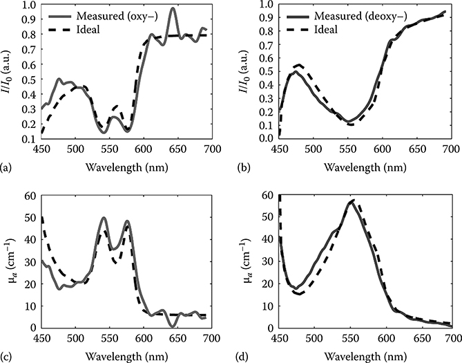
FIGURE 3.13
Measured absorption spectra for oxy-Hb (a) and deoxy-Hb (b) for concentrations of 50 and 68 g/L, respectively (solid lines). Dotted black lines are the theoretical predictions. Measured and theoretical attenuation coefficients for oxy-Hb (c) and deoxy-Hb (d). (Taken from Robles, F.E. et al., Biomed. Opt. Express, 1(1), 310, 2010.)
For biological samples, another important factor that influences absorption spectra is the oxygen saturation state of Hb. When including both oxy- and deoxy-Hb absorption, the attenuation coefficient can be written as where and CHb are the molar extinction coefficients and concentrations for oxy-/deoxy-Hb, respectively. Using the same formalism as with Equation 3.4, an overdetermined set of linear equations to solve for and CHb may be written as
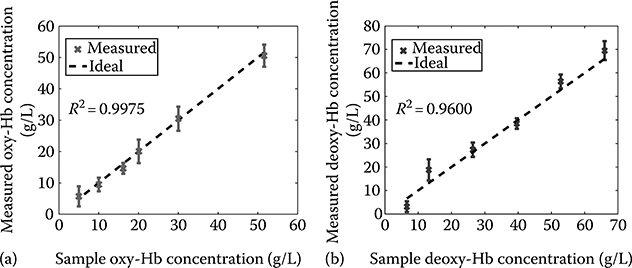
FIGURE 3.14
Measured Hb concentration for oxy- (a) and deoxy- (b) Hb samples. Error bars given by standard deviation across 25 measurements. Dotted black lines give the ideal trend with unity slope and zero intercept. (Taken from Robles, F.E. et al., Biomed. Opt. Express, 1(1), 310, 2010.)
where λi for 1 ≤ i ≤ n are the discretely measured wavelengths within the operating region. Finally, partial oxygen saturation (SO2) can be calculated as
The ability of our method to correctly measure oxygen saturation can be characterized by determining how well Equation 3.5 can be used to correlate measured data with the correct chromophore species. To determine the lowest concentration for which oxygen saturation states may be correctly measured, the correlation coefficient of the linear regression used to determine concentration in the previous analysis was calculated. Figure 3.15a shows the calculated correlation between the oxy-Hb data and the theoretical oxy- and deoxy-Hb extinction coefficients, and Figure 3.15b shows the same for the deoxy-Hb data.
Good agreement (R > 0.65) is observed for concentration values higher than 10 g/L if the data are compared to the correct species of Hb. A sharp cutoff can be seen below this point where the correlation coefficient drops drastically. From this analysis, we see that while concentration values may be determined as low as 1.2 g/L-mm, oxygenation states can only be accurately determined for concentrations above 4 g/L-mm (= 10 g/L × 0.4 mm).
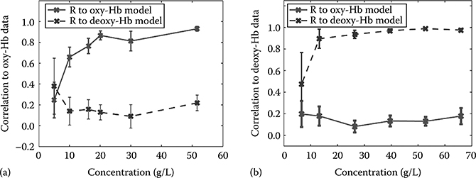
FIGURE 3.15
(a) Correlation coefficients between oxy-Hb data and ideal oxy-/deoxy-Hb extinction coeffi-cients at varying concentrations. (b) Correlation coefficients between the deoxy-Hb data and the oxy-/deoxy-Hb extinction coefficients at varying concentrations. Defining the detectable concentration as those with correlation coefficients greater than 0.65, a threshold of 4 g/L-mm is determined for accurately assessing oxygen saturation. (Taken from Robles, F.E. et al., Biomed. Opt. Express, 1(1), 310, 2010.)
Molecular imaging true color spectroscopic (METRiCS) OCT incorporates the imaging capabilities of OCT with the spectral analysis described earlier. While the analysis of Hb concentration and oxygenation state points to the utility of the method, it can also be applied to achieve molecular imaging of any absorber in the visible region of the spectrum, including endogenous and exogenous chromophores. In addition, because the system employs the visible region for imaging, the sample can be presented using its true colors offering an accessible, intuitive display of the spectroscopic information.
To demonstrate true color imaging, analysis of a sample consisting of a piece of paper with three lines, red, green, and blue, is presented. Figure 3.16a shows a photograph and pfdOCT image of the piece of paper. As previously noted, pfdOCT imaging reveal the structures of the samples, which in this case includes the indentation on the paper from the pens used to draw the lines; in addition, some absorption can be observed by the loss of intensity, particularly for the red and blue lines but spectral discrimination cannot be obtained by intensity analysis alone. To obtain the spectral information, each A-scan is processed with the DW method. Figure 3.16b shows the spectra from four points, labeled R, G, B, and W with arrows in Figure 3.16a. Here, the spectra were low pass filtered using a 7th-order Butterworth filter with a cutoff of 15 cycles. The spectrum obtained for a point below the red line (point labeled R) clearly shows a peak intensity at ∼630 nm, corresponding to what the human eye would perceive as red. Similarly, spectra obtained for points below the green and blue lines on the paper show peaks intensities at ∼524 and ∼460 nm, respectively; again, in good agreement with what the eye perceives for these colors. For completeness, a point corresponding to a white region is also plotted, and as expected, the spectrum spans all wavelengths.
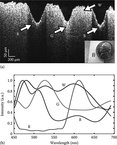
FIGURE 3.16
(a) pfdOCT image of a piece of paper with three lines drawn with colored pens, from left to right: red, green, and blue. Inset shows a photograph of the paper. (b) Spectra obtained with DW processing of OCT image from four points in the image from below the red (R), green (G), blue (B) line, and white (W) regions. (Taken from Robles, F.E., Light scattering and absorption spectroscopy in three dimensions using quantitative low coherence interferometry for biomedical applications, PhD thesis in Medical Physics, Duke University, Durham, NC, 2011.)
The ability to extract quantitative spectral information from each point of an image is a compelling strength of the DW approach. Thus, to easily interpret this wealth of spectroscopic information, the image can be represented using the sample's true colors by dividing each spectrum into three channels using the Commission Internationale d'Eclairage (CIE) color functions [43,44], which aligns with the chromatic response of the human eye. These functions are plotted in Figure 3.17 as compared with the spectrum of the light source. For image display of the spectral data, the interferograms are not normalized before processing with the DW method, as was done previously for quantifying the spectra. Omitting this step ensures that the RGB values are not polluted by noise, particularly in regions of low source intensity. Instead, image white balance is determined as follows [45]: First, the RGB values for each pixel are normalized. Then, the reciprocal average RGB values of a region with no expected spectral modulation are used to remove the influence (or color) of the source. Thus, a region with no absorption is assigned RGB values equal to 1. The result is a color-balanced hue map, which is then multiplied by the normalized pfdOCT image (saturation map) to yield a hue, saturation, and value (HSV) image, producing a true color representation of the sample. Figure 3.18 shows the true color image of the piece of paper produced by this process. Note that the image gives the same structural information as with pfdOCT, but now the colors provide access to the spectral information with an intuitive form of display.
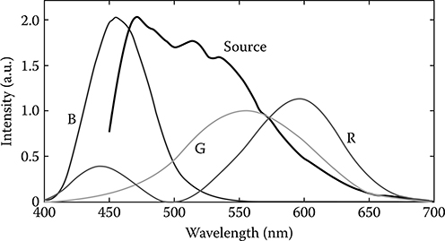
FIGURE 3.17
Commission Internationale d'Eclairage (CIE) color functions [44] and source spectrum.
To further define the imaging capabilities of METRiCS OCT, we consider a sample (Figure 3.19a) which consists of glass capillaries with ∼100 μm maximum outer diameter and ∼80 μm maximum inner diameter (Charles Supper, Natick, Ma), filled with red, green, and blue food-coloring dyes and immersed in agar and 2% intralipid (IL). IL is a fat emulsion that is often used as a model for scattering in tissue. Figure 3.19b shows the results of DW processing, where the absorption from the dyes in the capillaries is used to provide a true color display of the sample. A notable feature of this image is that spectral modulation is only observed from below the capillaries, where light is returned from scattering due to IL, owing to the fact that METRiCS OCT, as with conventional OCT, is only sensitive to the light returned from scatterers/reflectors. Note that no signal is present from within the capillaries, since the dyes do not scatter light. Here, spectral modulation is also observed due to the IL itself. This is due to its scattering cross section, which is proportional to λ−2.4, as described by van Staveren et al. [46], producing the yellow color at deeper sample depths. It is important to point out that METRiCS OCT is sensitive to the total attenuation coefficient, which includes absorption and scattering. However, for regions immediately following a significant amount of absorption, for example, below the capillaries, the color (and hence spectrum) is dictated primarily by the absorption coefficient.
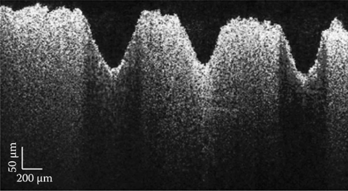
FIGURE 3.18
(See color insert.) True color OCT image of a paper with a red, green, and blue line. (Taken from Robles, F.E., Light scattering and absorption spectroscopy in three dimensions using quantitative low coherence interferometry for biomedical applications, PhD thesis in Medical Physics, Duke University, Durham, NC, 2011.)
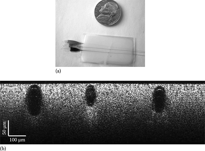
FIGURE 3.19 (See color insert.)
(a) Photograph and (b) METRiCS OCT image of tissue phantom consisting of intra-lipid and glass capillaries with food-color dyes. (Taken from Robles, F.E., Light scattering and absorption spectroscopy in three dimensions using quantitative low coherence interferometry for biomedical applications, PhD thesis in Medical Physics, Duke University, Durham, NC, 2011.)
To illustrate the utility of METRiCS OCT for imaging Hb in biological samples, we present images of chick embryos in vivo. For this preparation, a small window was made on the shells of eggs containing 4-day-old embryos, and then covered with tape. The embryos were kept in an incubator at ∼38°C and ∼80% humidity for 7 days. During this time, the embryos’ vasculature network grows considerably and thus serves as a good initial model to demonstrate METRiCS OCT's ability to provide molecular information from Hb absorption in vivo.
For the imaging experiments, the embryos were carefully removed from the shell (see Figure 3.20c) and placed on the motorized translational stage for imaging. While the pfd OCT system obtains x–z, B-mode images from a single exposure, the sample must be translated in the other (y) dimension to generate volumetric images. Figure 3.20a shows a B-mode, METRiCS OCT image of the chick empryo, and Figure 3.20b shows a 3D volume rendition of the entire data set. These samples contain a simple structure, consisting of the vasculature network around the yolk and the chorioallantoic membrane. As with the capillary phantom study presented previously, RBCs within the blood vessels impart a clear spectral modulation that is readily seen by the red shift in hue in locations below the vessels.
The full potential impact of this imaging method can be seen in the en face image, presented in Figure 3.21a. Here, several x–y planes are averaged to incorporate vessels found at different depths. This image clearly depicts the architecture of the vasculature network of the chick embryo, showing one major vessel, along with several branching vessels. Smaller capillaries are also seen, for example, in the upper left hand corner of Figure 3.21a. The significant advantage of METRiCS OCT is that not only is color information available but also that full detailed spectral profiles may be quantitatively analyzed. Figure 3.21b through e shows spectra from four selected points (solid black lines), along with the ideal molar extinction coefficient (red lines) for each measured Hb oxygen level. For this analysis, it is assumed that, for regions below the blood vessels, absorption is the dominant effect such that the method described earlier (Equations 3.2–3.6) may be applied to quantify the Hb oxygen levels (Figure 3.21). Note that the dotted lines are presented for only the limited bandwidth used for calculating SO2, since this region inherently provides an orthogonal basis set. The results suggest that the major vessel in this image is an artery, where points c–d contain varying levels of oxygenated Hb. In contrast, the analysis for the smaller vessel, indicated by point (b), shows that it contains deoxygenated Hb.

FIGURE 3.20
METRiCS OCT, B-mode image (a) and 3D volume (b) of a chick embryo. White x and z scale bars, 100 μm. Photograph of the sample (c). (Taken from Robles, F.E., Light scattering and absorption spectroscopy in three dimensions using quantitative low coherence interferometry for biomedical applications, PhD thesis in Medical Physics, Duke University, Durham, NC, 2011.)
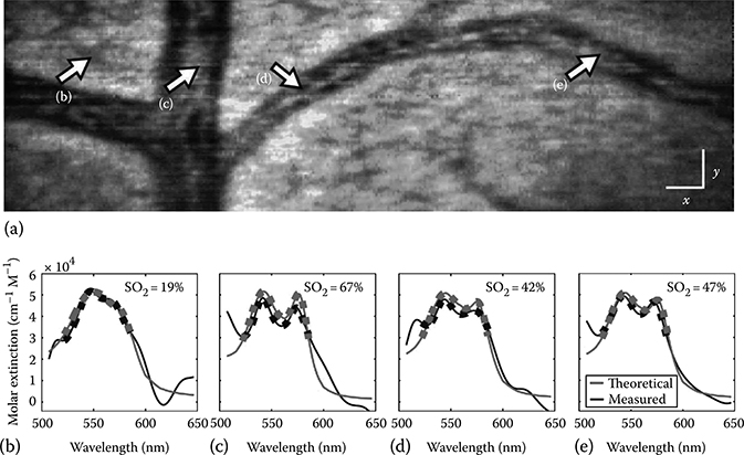
FIGURE 3.21
(a) En face METRiCS OCT image of chick embryo. White x and y scale bars, 100 μm. (b)–(e) Measured and theoretical spectral profiles from points (b)–(e), along with the computed Hb oxygen saturation. (Taken from Robles, F.E., Light scattering and absorption spectroscopy in three dimensions using quantitative low coherence interferometry for biomedical applications, PhD thesis in Medical Physics, Duke University, Durham, NC, 2011.)
As a final demonstration of the capabilities of METRiCS OCT, we present images acquired in vivo from a CD1 nu/nu normal mouse dorsal skinfold window chamber model [47]. Molecular contrast is demonstrated in this model for both endogenous and exogenous contrast. For imaging of endogenous contrast due to Hb absorption, the mouse was anesthetized and the window chamber was removed for imaging. Conventional OCT imaging of the data reveals tissue structures, as seen in Figure 3.22a. Here, several histological structures are evident, including the muscle layer, the lumen of blood vessels—including small capillaries—and the subcutaneous layer [48]. However, functional information regarding the sample is not available in this format. Using METRiCS OCT (Figure 3.22b), the spectral information reveals several interesting features: for example, the muscle layer at the surface appears relatively colorless due to low concentration of Hb, but once light traverses through the vasculature network beneath, a red shift is clearly observed due to higher concentrations of Hb. Another interesting feature is the small color variations on the top layer due to scattering from muscle and fibrous structures. Moreover, in regions below large blood vessels (>100 μm), most of the light is attenuated, thereby preventing detection of signals from below and thus creating a “shadow” effect. However, in regions without apparent blood vessels, signals are obtained throughout the full penetration depth enabled by the system.
Similar to the chick embryo results, the en face image, shown in Figure 3.23a, provides a more global perspective of the vasculature network. This image shows two major vessels, with the larger one on the right corresponding to a vein and the other to an artery. Several branching vessels can also be observed, along with the capillary plexus. Again, four points of interest are selected to analyze the spectra quantitatively; these points are found along a vbranching vessel from the vein (Figure 3.23b), two from the artery (Figure 3.23c and d), and from the capillary network (Figure 3.23e). As Figure 3.23b through e shows, the measured spectra are well fit by the theoretical model and the calculated SO2 levels, shown in the figure, correspond to expected values for these tissue locations in the anesthetized mouse [50].

FIGURE 3.22
Tomographic (x–z) images of mouse dorsal skin flap. (a) Conventional OCT image and (b) METRiCS OCT image, demonstrating endogenous contrast molecular imaging. The white x and z scale bars are 100 μm. (Taken from Robles, F.E. et al., Nat. Photon., 5(12), 744, 2011.)

FIGURE 3.23
(a) En face (x–y) METRiCS OCT image using endogenous contrast, with arrows indicating points where the spectra presented in (b)–(e) are quantified. The white x and y scale bars are 100 μm. The measured spectral profiles are superposed with the theoretical Hb molar extinction coefficients. The dotted portion of the curves outlines the region used to determine SO2 levels. All spectra were selected from depths immediately beneath each corresponding vessel. (Taken from Robles, F.E. et al., Nat. Photon., 5(12), 744, 2011.)
To show the variations across individual vessels, Figure 3.24 shows a B-mode METRiCS OCT image and spectral analysis from the same data set (point b in Figure 3.23). Figure 3.24b through d presents spectra sampled across the diameter of this vessel with low oxygen levels, whereas (e–f) show spectra sampled longitudinally along a vessel with higher oxygen saturation levels. In both vessels, relatively small variations of only a few percent in saturation are observed.
Finally, imaging using an exogenous contrast agent, an area that has seen limited success in OCT to date, is presented. Here, 100 μL of sodium fluores-cein (NaFS), diluted in sterile saline to 1% by weight, was introduced via a retro orbital injection, an intravenous injection which is an alternative to a tail vein injection. The images (Figures 3.25 and 3.26) clearly depict the presence of NaFS by a strong red shift in hue, which arises from stronger absorption at the lower wavelengths compared to that observed with endogenous contrast. Note that the injection results in the agent remaining confined to the vessels as it does not extravasate appreciably. Surprisingly, the agent also shows a weak increase in scattering. As a result, vessels are now char-acterized by the red hue of NaFS in the en face image (Figure 3.26a); however, large vessels still exhibit a “shadow” due to the stronger absorption.
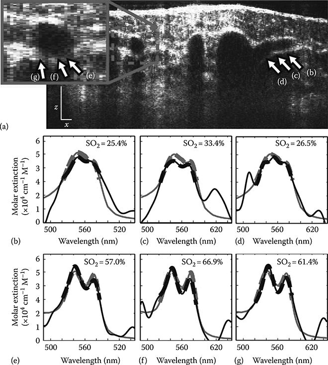
FIGURE 3.24
Tomographic (x–z) METRiCS OCT image of mouse dorsal skin flap with a close up of a vessel, and corresponding spectral profiles. (a) Cross-sectional image, acquired for point (b) in Figure 3.24. The white x and z scale bars are 100 μm. (b)–(d), Spectral profiles from points (b)–(d), sampled across the diameter of a deoxygenated vessel. (e)–(f), Spectral profiles from points (e)–(f), sampled longitudinally along a vessel with higher oxygen saturation levels. (Taken from Robles, F.E. et al., Nat. Photon., 5(12), 744, 2011.)
Spectra from four points of interest are selected (Figure 3.26b through e), where the contributions of the three absorbing species (oxy-Hb, deoxy-Hb, and NaFS) are seen to affect the localized spectra to varying degrees. As shown in Figure 3.26b through e, the presence of NaFS only contributes to the attenuation spectra in the lower wavelengths, thus assessment of SO2 may still be accomplished as described previously. The relative amount of absorption due to NaFS with respect to total Hb (∊ ≡ NaFS/Hb) is also computed. The results show that this ratio is relatively constant (∼1), which is expected since both NaFS and Hb are contained within the vessels and their relative contributions with respect to one another should not vary appreciably from location to location.

FIGURE 3.25
Tomographic (x–z) images of mouse dorsal skin flap window with exogenous contrast due to sodium fluorescein injection. (a) Conventional OCT image and (b) METRiCS OCT image, located above point (e) as shown in the en face (x–y) image in Figure 5.26. The white x and z scale bars are 100 μm. (Taken from Robles, F.E. et al., Nat. Photon., 5(12), 744, 2011.)
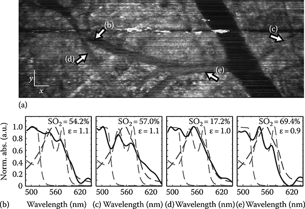
FIGURE 3.26 (See color insert.)
(a) En face (x–y) METRiCS OCT image of mouse dorsal skin flap window using exogenous contrast, and (b) spectral profiles from points indicated by arrows. The white x and y scale bars are 100 μm. The measured spectral profiles (black) are superposed with the theoretical oxy- (dotted red) and deoxy- (dotted blue) Hb normalized extinction coefficients, and normalized absorption of NaFS (dotted green). Also shown are the SO2 levels and relative absorption of NaFS with respect to total Hb (∊ ≡ NaFS/Hb). All spectra were selected from depths immediately beneath each corresponding vessel. (Taken from Robles, F.E. et al., Nat. Photon., 5(12), 744, 2011.)
A final observation of this data shows an apparent effect of detector saturation due to fluorescent light from the NaFS, as the green areas of the en face image (Figure 3.26). The contrast agent (NaFS) absorbs light with maximum efficiency around 494 nm, producing the red hue of the vessels in the METRiCS OCT images. However, it also emits incoherent fluorescent light at a peak wavelength of 521 nm (green light). When this signal is particularly strong, green spots are seen in the image where the detector is saturated due to the fluorescent green signal.
3.5 Discussion
The development of fLCI and METRiCS OCT are a significant advance in the biomedical optics field due to the ability to provide depth resolved spectral information within an OCT image. The basis of this advance arises from the DW method, due to its ability to provide simultaneously high spectral and spatial resolution from interferometric signals. As described earlier, the DW method combines two linear time frequency distributions, each with different spatial and spectral properties, to form a new type of bilinear distribution. It has been shown mathematically [12] that the DW method probes the Wigner bilinear distribution with two orthogonal, independent windows, thus overcoming the resolution trade-off associated with linear distributions and avoiding common artifacts found in bilinear distributions.
The DW method served as a powerful tool for advance fLCI, enabling scattering signatures to be analyzed via depth resolved spectra to identify structures that were not resolved in the traditional OCT image. This method analyzes high-frequency oscillations of local spectra, resulting from induced temporal coherence effects, to determine the size of dominant scatterers. Analysis of these spectral features in complex, three-dimensional samples was not possible prior to the DW method due to the requirement for high resolution in both the spectral and the spatial dimensions. However, with the DW method, the local oscillations could be recovered and quantitative analysis was enabled. This capability was demonstrated using a phantom consisting of agar and polystyrene microspheres of different sizes in two distinct layers as a model of how cell nuclei may be distributed in different layers of tissue. Experiments with an ex vivo rat carcinogenesis model provided a powerful demonstration of fLCI's ability to detect early signs of cancerous development, with the cell nuclear diameter used as a surrogate biomarker of disease. The DW fLCI approach was shown to distinguish between normal and treated tissues, and provided evidence of the field effect of carcinogenesis.
The DW method was also used to gain access to spatially varying spectral modulations due to absorption. Unlike the local oscillations in fLCI, absorption from chromophores, such as Hb, produce a spectral modulation that is lower in frequency, thereby permitting facile separation of the two effects. With METRiCS OCT, molecular information of endogenous and exogenous chromophores is provided alongside structural information. The visible region of the spectrum affords highly sensitive measurements to biologically relevant chromophores, such as Hb and many exogenous absorbers in the visible region of the spectrum. This is important because a vast number of previously developed fluorophores, such as FDA-approved NaFS, may be leveraged for functional, tomographic imaging. METRiCS OCT not only provides contrast of these molecules but also has been shown to quantify SO2 levels in vivo. Lastly, by having access to the full visible spectrum, an intuitive form of display using sample's true colors was achieved.
The optical imaging tools described here enable a number of different applications in biomedicine, each facing their own unique challenges in translation that will direct future work. In fLCI, an optical fiber-based system is needed to apply the method in vivo. Automated algorithms that contour the surface of tissues will facilitate analysis of large data sets corresponding to wide areas of tissue. The advantage of using fLCI is that processed data obtained from the images avoid the need to be interpreted by trained experts. The results presented here show that fLCI can assess tissue health quantitatively and provide sensitivity to precancerous states offering a potential new avenue for screening and diagnosing cancer.
Future work on METRiCS OCT will focus on application to animal models, in an effort to understand biological processes such as tumorigenesis and to identify changes to assess efficacy of therapeutic interventions. Although METRiCS OCT has only been demonstrated recently, the results show that it is a powerful tool that could enable new directions in early cancer detection, monitoring the delivery of therapeutic agents, and fundamental research, such as improving the understanding of angiogenesis and hypoxia.
Acknowledgment
This work was supported by a grant from the National Institutes of Health through the National Cancer Institute (1 R01 CA 138594).
References
1. Huang, D., E.A. Swanson, C.P. Lin, J.S. Schuman, W.G. Stinson, W. Chang, M.R. Hee, T. Flotte, K. Gregory, C.A. Puliafito, and J.G. Fujimoto, Optical coherence tomography. Science, 1991. 254(5035): 1178–1181.
2. Huang, D., Y. Li, and M. Tang, Anterior eye imaging with optical coherence tomography, in Optical Coherence Tomography: Tenchology and Applications, W. Drexler and J. Fujimoto, eds. 2008. Springer, New York.
3. Wojtkowski, M., R. Leitgeb, A. Kowalczyk, T. Bajraszewski, and A. Fercher, In vivo human retinal imaging by Fourier domain optical coherence tomography. J. Biomed. Opt., 2002. 7: 457.
4. Choma, M., M. Sarunic, C. Yang, and J. Izatt, Sensitivity advantage of swept source and Fourier domain optical coherence tomography. Opt. Express, 2003. 11(18): 2183–2189.
5. Robles, F.E., Light scattering and absorption spectroscopy in three dimensions using quantitative low coherence interferometry for biomedical applications, PhD thesis in Medical Physics. 2011. Duke University, Durham, NC.
6. Morgner, U., W. Drexler, F. Kärtner, X. Li, C. Pitris, E. Ippen, and J. Fujimoto, Spectroscopic optical coherence tomography. Opt. Lett., 2000. 25(2): 111–113.
7. Faber, D., E. Mik, M. Aalders, and T. van Leeuwen, Toward assessment of blood oxygen saturation by spectroscopic optical coherence tomography. Opt. Lett., 2005. 30(9): 1015–1017.
8. Yi, J. and X. Li, Estimation of oxygen saturation from erythrocytes by high-resolution spectroscopic optical coherence tomography. Opt. Lett., 2010. 35(12): 2094–2096.
9. Cang, H., T. Sun, Z. Li, J. Chen, B. Wiley, Y. Xia, and X. Li, Gold nanocages as contrast agents for spectroscopic optical coherence tomography. Opt. Lett., 2005. 30(22): 3048–3050.
10. Oldenburg, A., M. Hansen, T. Ralston, A. Wei, and S. Boppart, Imaging gold nanorods in excised human breast carcinoma by spectroscopic optical coherence tomography. J. Mater. Chem., 2009. 19: 6407.
11. Faber, D.J. and T.G.v. Leeuwen, Are quantitative attenuation measurements of blood by optical coherence tomography feasible? Opt. Lett., 2009. 34: 1–3.
12. Robles, F., R.N. Graf, and A. Wax, Dual window method for processing spectroscopic optical coherence tomography signals with simultaneously high spectral and temporal resolution. Opt. Express, 2009. 17(8): 6799–6812.
13. Wang, X., B. Pogue, S. Jiang, X. Song, K. Paulsen, C. Kogel, S. Poplack, and W. Wells, Approximation of Mie scattering parameters in near-infrared tomography of normal breast tissue in vivo. J. Biomed. Opt., 2005. 10(5): 051704.
14. Drezek, R., M. Guillaud, T. Collier, I. Boiko, A. Malpica, C. Macaulay, M. Follen, and R. Richards-Kortum, Light scattering from cervical cells throughout neoplastic progression: influence of nuclear morphology, DNA content, and chromatin texture. J. Biomed. Opt., 2003. 8(1): 7.
15. Seet, K., T. Nieminen, and A. Zvyagin, Refractometry of melanocyte cell nuclei using optical scatter images recorded by digital Fourier microscopy. J. Biomed. Opt., 2009. 14(4): 044031.
16. Graf, R., F.E. Robles, X. Chen, and A. Wax, Detecting precancerous lesions in the hamster cheek pouch using spectroscopic white–light optical coherence tomography to assess nuclear morphology via spectral oscillations. J. Biomed. Opt., 2009. 14: 064030.
17. Wax, A., C. Yang, and J. Izatt, Fourier-domain low-coherence interferometry for light-scattering spectroscopy. Opt. Lett., 2003. 28(14): 1230–1232.
18. Graf, R. and A. Wax, Nuclear morphology measurements using Fourier domain low coherence interferometry. Opt. Express, 2005. 13(12): 4693–4698.
19. Perelman, L.T., V. Backman, M. Wallace, G. Zonios, R. Manoharan, A. Nusrat, S. Shields, M. Seiler, C. Lima, T. Hamano, I. Itzkan, J. Van Dam, J.M. Crawford, and M.S. Feld, Observation of periodic fine structure in reflectance from biological tissue: A new technique for measuring nuclear size distribution. Phys. Rev. Lett., 1998. 80(3): 627–630.
20. van de Hulst, H.C., Light Scattering by Small Particles. 1981. Dover Publications, New York.
21. Robles, F.E. and A. Wax, Measuring morphological features using light-scattering spectroscopy and Fourier-domain low-coherence interferometry. Opt. Lett., 2010. 35(3): 360–362.
22. Wax, A., C.H. Yang, V. Backman, K. Badizadegan, C.W. Boone, R.R. Dasari, and M.S. Feld, Cellular organization and substructure measured using angle-resolved low-coherence interferometry. Biophys. J., 2002. 82(4): 2256–2264.
23. Reddy, B.S., Studies with the azoxymethane-rat preclinical model for assessing colon tumor development and chemoprevention. Environ. Mol. Mutagen., 2004. 44(1): 26–35.
24. Roy, H.K., A. Gomes, V. Turzhitsky, M.J. Goldberg, J. Rogers, S. Ruderman, K.L. Young , Spectroscopic microvascular blood detection from the endoscopi-cally normal colonic mucosa: Biomarker for neoplasia risk. Gastroenterology, 2008. 135(4): 1069–1078.
25. Kim, Y.L., V.M. Turzhitsky, Y. Liu, H.K. Roy, R.K. Wali, H. Subramanian, P. Pradhan, and V. Backman, Low-coherence enhanced backscattering: review of principles and applications for colon cancer screening. J. Biomed. Opt., 2006. 11(4): 041125.
26. Braakhuis, B.J.M., M.P. Tabor, J.A. Kummer, C.R. Leemans, and R.H. Brakenhoff, A genetic explanation of Slaughter's concept of field cancerization: Evidence and clinical implications. Cancer Res., 2003. 63(8): 1727–1730.
27. Zysk, A.M., S.G. Adie, J.J. Armstrong, M.S. Leigh, A. Paduch, D.D. Sampson, F.T. Nguyen, and S.A. Boppart, Needle-based refractive index measurement using low-coherence interferometry. Opt. Lett., 2007. 32(4): 385–387.
28. Robles, F., Y. Zhu, J. Lee, S. Sharma, and A. Wax, Fourier domain low coherence interferometry for detection of early colorectal cancer development in the azoxy-methane rat carcinogenesis model. Biomed. Opt. Express, 2010. 1(2): 736–745.
29. Choi, W., C. Fang-Yen, K. Badizadegan, S. Oh, N. Lue, R.R. Dasari, and M.S. Feld, Tomographic phase microscopy. Nat. Methods, 2007. 4(9): 717–719.
30. Brown, W.J., J.W. Pyhtila, N.G. Terry, K.J. Chalut, T. D'Amico, T.A. Sporn, J.V. Obando, and A. Wax, Review and recent development of angle-resolved low coherence interferometry for detection of pre-cancerous cells in human esophageal epithelium. IEEE J. Sel. Top. Quant Electron, 2008. 14: 88–97.
31. Terry, N.G., Y. Zhu, M.T. Rinehart, W.J. Brown, S.C. Gebhart, S. Bright, E. Carretta , Detection of dysplasia in Barrett's esophagus with in vivo depth-resolved nuclear morphology measurements. Gastroenterology, 2011. 140(1): 42–50.
32. Terry, N.G., Y.Z. Zhu, J.K.M. Thacker, J. Migaly, C. Guy, C.R. Mantyh, and A. Wax, Detection of intestinal dysplasia using angle-resolved low coherence interferometry. J. Biomed. Opt., 2011. 16(10): 106002.
33. Wax, A., J.W. Pyhtila, R.N. Graf, R. Nines, C.W. Boone, R.R. Dasari, M.S. Feld, V.E. Steele, and G.D. Stoner, Prospective grading of neoplastic change in rat esophagus epithelium using angle-resolved low-coherence interferometry. J. Biomed. Opt., 2005. 10(5): 051604.
34. Wax, A., C. Yang, M.G. Müller, R. Nines, C.W. Boone, V.E. Steele, G.D. Stoner, R.R. Dasari, and M.S. Feld, In situ detection of neoplastic transformation and chemopreventive effects in rat esophagus epithelium using angle-resolved low-coherence interferometry. Cancer Res., 2003. 63(13): 3556.
35. Ntziachristos, V., C.H. Tung, C. Bremer, and R. Weissleder, Fluorescence molecular tomography resolves protease activity in vivo. Nat. Med., 2002. 8(7): 757–761.
36. Wang, X., Y. Pang, G. Ku, X. Xie, G. Stoica, and L.V. Wang, Noninvasive laser-induced photoacoustic tomography for structural and functional in vivo imaging of the brain. Nat. Biotechnol., 2003. 21(7): 803–806.
37. Helmchen, F. and W. Denk, Deep tissue two-photon microscopy. Nat. Methods, 2005. 2(12): 932–940.
38. Boppart, S.A., A.L. Oldenburg, C. Xu, and D.L. Marks, Optical probes and techniques for molecular contrast enhancement in coherence imaging. J. Biomed. Opt., 2005. 10: 041208.
39. Graf, R., W. Brown, and A. Wax, Parallel frequency-domain optical coherence tomography scatter-mode imaging of the hamster cheek pouch using a thermal light source. Opt. Lett., 2008. 33(12): 1285–1287.
40. Prahl, S. Optical Absorption of Hemoglobin 1999; Available from: http://omlc.ogi.edu/spectra/hemoglobin/.
41. Robles, F.E., S. Chowdhury, and A. Wax, Assessing hemoglobin concentration using spectroscopic optical coherence tomography for feasibility of tissue diagnostics. Biomed. Opt. Express, 2010. 1(1): 310–317.
42. Wang, H., J. Jiang, C. Lin, J. Lin, G. Huang, and J. Yu, Diffuse reflectance spectroscopy detects increased hemoglobin concentration and decreased oxygenation during colon carcinogenesis from normal to malignant tumors. Opt. Express, 2009. 17(4): 2805–2817.
43. Selected Colorimetric Tables. 2011; Available from: http://www.cie.co.at.
44. Boppart, S.A., A. Goodman, J. Libus, C. Pitris, C.A. Jesser, M.E. Brezinski, and J.G. Fujimoto, High resolution imaging of endometriosis and ovarian carcinoma with optical coherence tomography: feasibility for laparoscopic-based imaging. Br. J. Obstet. Gynaecol., 1999. 106(10): 1071–1077.
45. lves, H.E., The relation between the color of the llluminant and the color of the illuminated object. Trans. Ilium. Eng. Soc., 1912. 7: 62–72.
46. van Staveren, H., C. Moes, J. van Marie, S. Prahl, and M.J.C. van Gemert, Light scattering in Intralipid-10% in the wavelength range of 400–1100 nm. Appl. Opt., 1991. 30(31): 4507–4514.
47. Huang, Q., S. Sha, R.D. Braun, J. Lanzen, G. Anyrhambatla, G. Kong, M. Borelli, P. Corry, M.W. Dewhirst, and C.Y. Li, Noninvasive visualization of tumors in rodent dorsal skin window chambers. Nat. Biotechnol., 1999. 17(10): 1033–1035.
48. Koehl, G.E., A. Gaumann, and E.K. Geissler, Intravital microscopy of tumor angiogenesis and regression in the dorsal skin fold chamber: mechanistic insights and preclinical testing of therapeutic strategies. Clin. Exp. Metastasis, 2009. 26(4): 329–344.
49. Robles, F.E., C. Wilson, G. Grant, and A. Wax, Molecular imaging true-colour spectroscopic optical coherence tomography. Nat. Photon., 2011. 5(12): 744–747.
50. Skala, M.C., A. Fontanella, L. Lan, J.A. Izatt, and M.W. Dewhirst, Longitudinal optical imaging of tumor metabolism and hemodynamics. J. Biomed. Opt., 2010. 15: 011112.