
CHAPTER 10
Mobile-Robot Navigation
CONTENTS
10.4 Modifying navigation stack
Introduction To this point, consideration of planning has been restricted to point-and-move along some specified polyline. More generally, a vehicle should be able to plan and execute its own motion toward a goal destination. In doing so, it should consider all a priori information available, such as a pre-recorded map, as well as unexpected obstacles encountered en route. In ROS, this is addressed with what is often referred to as the navigation stack.
The navigation stack assumes use of maps, localization, and obstacle sensing. With specifications of vehicle dimensions, costmaps representing poses in the environment as having corresponding penalties are computed. A global planner computes collision-free paths from the robot’s current pose to a specified goal destination. While following a global path plan, the robot senses and responds to obstacles, typically resulting in path deviations that bypass the obstacle and re-join the global plan.
In this chapter, use of the navigation stack via the package is introduced. We start with describing a process for map making, then show how maps can be used with the nav-stack and how action clients can invoke the functionality of the nav-stack.
10.1 Map making
The package can be used to create maps using a mobile robot and a LIDAR sensor. Per the wiki, http://www.w3.org/1999/xlink:
The package provides laser-based SLAM (Simultaneous Localization and Mapping), as a ROS node called . Using , you can create a 2-D occupancy grid map (like a building floorplan) from laser and pose data collected by a mobile robot.
To use this package, the robot’s LIDAR must be mounted horizontally with a fixed mount, and the robot must publish odometry. This package post-processes LIDAR and data and attempts to build a map that explains the LIDAR data relative to the robot’s movements.
Mapping can be performed online, or as a post-process. For the post-processing approach, the first step in map making is to acquire (bag) data. As an example, start Gazebo:

The file in the package starts the mobot model, brings in the model, starts the desired-state publisher, and starts an open-loop controller. The robot model used in this launch contains LIDAR, a Kinect sensor and a color camera. is also launched. Perform these operations with:

With the robot running, should show that the LIDAR is active and that it can sense the walls of the starting pen. At this point, the robot should wander (slowly) through some path, exploring its environment while bagging data on the topics and (where is the LIDAR topic for the mobot model).
To record the data, navigate to a desired directory. The current example uses the directory within the repository. From the chosen directory, start recording data with:

While data is being recorded, have the robot move. An example pre-scripted motion for a 3 m 3 m square path may be invoked with:

If desired, this can be re-run to have the robot perform a second (or third) repeat of the path. Due to open-loop control, the robot will drift from the desired path, so repeats of this path request will yield novel viewpoints, which are useful for map making.
When using a real robot for map making, one can start the bagging process, then use a joystick to manually drive the robot through the environment of interest. When doing so, one should take care to move the robot slowly, particularly in turning motions. Such data will be easier to post-process to reconcile scans from different poses.
Once enough data has been collected, kill the process (with control-C). Gazebo can be killed as well. The bagged data will be contained in the file within the chosen directory.
Given a recording that contains LIDAR scan data and transform ( ) data, the can be post-processed to compute a corresponding map. To do so, start a roscore, then, from the directory in which the data resides, run:

The remapping option is not necessary in the present example, since the LIDAR scan topic for the mobot model is already called . However, if the robot’s scan topic were, e.g. , one should use topic re-mapping with the option: . At this point, the map builder is subscribed to the topic and to the LIDAR topic. To publish the acquired data to the respective topics, playback the data with:

The above command assumes that the recorded data is called (an option chosen during recording), and it is assumed that this command is run from the directory in which resides. With both and running, the map making node will receive publications of LIDAR and data and will attempt to build a map from this data.
The map making process can be watched dynamically, if desired. To do so, bring up :

Add a display item. In the display panel, expand this new item and choose the topic . While the recording is played back, one can watch a display of the map being built.
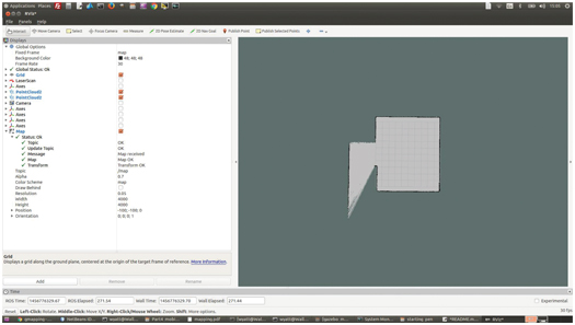
Figure 10.1 rviz view of map constructed from recorded data of mobot moving within starting pen
Figure 10.1 shows an example 2-D occupancy map in which shades of gray imply the degree of certainty of
a cell being occupied. Black cells correspond to high probability of occupancy, and white cells imply a high probability of being vacant. Gray cells imply no information is available. The display in Fig 10.1 is a credible fit to the starting pen. The exit hallway is incompletely mapped, since the robot did not travel to poses from which a line-of-sight LIDAR acquisition could detect the occluded hallway.
When the bag-file playback is complete, the created map needs to be saved to disk. This is done with the command:

where is the file name, which should be chosen mnemonically. This will create two files: and . For the example map created, the file contains:
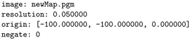
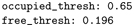
These parameters declare that the map data can be found in the file named , and that the resolution of cells within this map is 5 cm. The threshold values are used by planning algorithms to decide whether a cell is to be called occupied or vacant.
The map data is contained in . This is in an image format, which can be viewed directly just by double-clicking the file within Linux. If desired, the map may be touched up using an image editor program.
As an alternative to logging (bagging) data and post-processing to create a map, the map making can be performed interactively. To do so, one should start a robot in an environment of interest, and make sure that the LIDAR sensor is active, that its transform to the robot’s base frame is published, that odometry is published, and that the robot is prepared to be moved under teleoperation. For our simulated mobile robot, this can be accomplished using:

This launch file starts Gazebo, spawns a model of the starting pen, loads the mobot model onto the parameter server, spawns the robot model into Gazebo, and starts a robot-state publisher. In the present case, the LIDAR link is already part of the robot model, and thus its transform to the robot-base frame will be published by the robot-state publisher. When running a physical robot, a static transform publisher would be needed to establish the pose of the LIDAR relative to the robot’s base frame.
With the robot started in the environment of interest, three nodes should be run: , and (or some equivalent means to command the robot). These nodes can be started with assistance of a launch file in the package :

This launch file launches using a stored configuration file that includes a display (on topic ). When these nodes are launched, the display appears as in Fig 10.2.

Figure 10.2 Initial view of gmapping process with mobot in starting pen
As the robot moves through its environment, more of the map is constructed. Figures 10.3 through 10.5 show the evolution of the map as the robot turns slightly counter-clockwise, after a full revolution, then after beginning to enter the exit hallway.
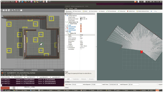
Figure 10.3 Map after slight counter-clockwise rotation

Figure 10.4 Map after full rotation
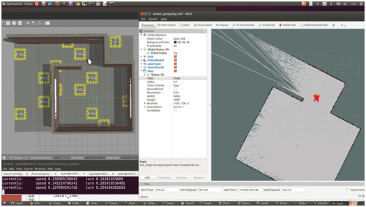
Figure 10.5 Map state as robot first enters exit hallway
The starting pen map in , as previously invoked in Fig 9.15, was constructed by this process, including having the robot exit the starting pen and encircle the pen to establish both interior and exterior map representations.
It was shown in Section 9.2.4 that a map can be used to help establish a robot’s pose relative to that map. In addition, having a map supports making motion plans, as will be described next.
10.2 Path planning
One of the most commonly used packages in ROS is , which incorporates many features. The node incorporates global planning, local planning and steering. Global and local planning are based on the notion of costmaps, described at http://www.w3.org/1999/xlink.
An example costmap can be visualized by starting up the mobot model in the starting pen:

then running :

This launch file loads the starting pen map (with ), starts , starts with a preset configuration, and starts with multiple configuration settings (which will be discussed in detail).
The above launch produces the view of Fig 10.6. This display shows the map of the starting pen, construction of which was described in Section 10.1. The overlay of red dots corresponding to LIDAR pings shows that successfully localized the robot with respect to the map, since the LIDAR pings line up with walls within the map.
Additionally, the map’s walls have a fattened, colorized border. These borders correspond to cost penalties, encoded as color. To use the costmap, one defines a footprint for the robot (as part of the configuration). For planning purposes, a candidate path solution is penalized for allowing non-zero cost cells to be contained within the robot’s footprint. Moving close to a barrier may be acceptable, but at some modest cost. However, allowing a forbidden (lethal) cell within the footprint would score a candidate path as non-viable. The gray areas of the map carry no penalty, and path solutions that keep the robot’s footprint entirely within the non-colored regions have the lowest penalty assigned.

Figure 10.6 Global costmap of starting pen
Figure 10.7 shows an example of global path planning with respect to the fattened map. The blue trace displays the plan computed by the global planner. The goal for this example was set interactively through use of the tool in . By clicking this tool, then clicking and dragging the
mouse somewhere within an unoccupied region of the map, one can set both the origin and heading of a navigation goal. In Fig 10.7, the goal thus set is displayed as a frame (colored triad). The path displayed keeps a buffer distance from all walls while trying to reach the goal in minimum distance. A local planner (incorporating a steering algorithm) is responsible for driving the robot along the proposed path solution.
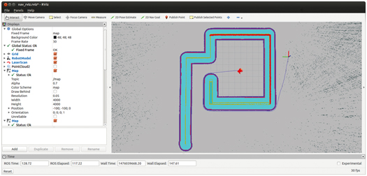
Figure 10.7 Global plan (blue trace) to specified 2dNavGoal (triad)
Global path solutions are computed with respect to a known map. However, unexpected barriers can invalidate the plan. For this reason, a local costmap is also computed and interpreted.
Figure 10.8 shows a local costmap overlaid on the global costmap.
In this case, a barrier (a construction barrel) was added to Gazebo in front of the robot. This obstacle was not present during the original mapping process, and thus it is unknown to the global costmap. Such cases are commonplace, as furniture may be rearranged, pallets may be moved about a factory, or people, vehicles or other robots may appear unexpectedly as obstacles. As shown in Fig 10.8, the local costmap is myopic; it is only aware of obstacles sensed within some defined window relative to the robot. Although the sensor may have longer range, the local costmap is deliberately represented as a short-range interpretation. In Fig 10.8, the barrel has only just entered the robot’s local awareness.

Figure 10.8 Global and local costmaps with unexpected obstacle (construction barrel)
As the barrier is detected, the path plan is re-generated to go around the obstacle, as shown by the blue trace in Fig 10.8.
From this brief introduction, it is apparent that much computation is occurring behind the scenes. Further, considerable tuning is required to obtain good performance. Tuning is prescribed using four configuration files: , , and . Setting configuration parameters for the nav-stack is described in http://www.w3.org/1999/xlink, and in greater detail in http://www.w3.org/1999/xlink for costmap parameters and http://www.w3.org/1999/xlink for planning parameters.
For our example mobot, these files reside in the package . The file contains:

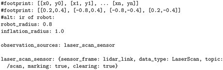
These parameters specify that the LIDAR sensor data will have a limit of awareness of obstacles only out to 3.0 m, and that clearing of obstacles may occur out to 3.5 m. (Obstacles are cleared by recognizing that a LIDAR ray extends beyond some threshold radius, and thus there are no obstacles along that ray out to the threshold radius.) A footprint may be defined either by specifying coordinates of a polygon (expressed in the
robot’s base frame), or by specifying a simple radius about the robot’s base frame origin. In the present case, the commented-out polygon is a reasonable approximation to the outline of the mobot. However, planning with respect to a polygon is more complex than planning with respect to a circle–particularly since the mobot’s origin (between the drive wheels) is significantly offset from the center of the bounding rectangle. The alternative of setting a radius must be conservative in order to enclose the full outline of the robot (particularly since the robot’s origin is not in the center of the robot’s footprint). Assuming a conservative circular boundary simplifies planning and leads to fewer deadlock conditions. However, such a conservative boundary also prevents finding viable plans through narrow (but feasible) passageways.
An inflation radius of 1 m is also quite conservative. Plans will be penalized for coming closer than this to walls and other obstacles.
The field should contain all sensors that will be used for obstacle detection.
Most commonly (as in this case), a LIDAR will be used. Various depth camera types are also options. Such sensors have the benefit of being aware of obstacles that do not appear in a 2-D LIDAR’s slice plane. For each sensor type listed, one must also specify the sensor frame and the sensor’s message type. Dynamic local costmaps are marked by sensing obstacles and cleared by sensing empty space. Marking and clearing will ordinarily be enabled by setting these fields to .
The parameters set within are applied to both global and local planning. Additional parameters are specific to the global and local planners. The file is shown below:
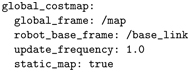
This file specifies that global planning should be performed in the frame, and the robot’s path will be specified with respect to its frame. For the global planner to succeed, a transform must be published between the and the frame. If a map is loaded and if is running, this transform will be published by . If these frames have been assigned other names, the names must be reflected in the configuration file. The parameter has been set to to recognize that a full map has already been obtained and loaded. In contrast, a map that is being constructed dynamically, e.g. using SLAM, would not be static.
Costmap parameters specific to the local planner are specified in , shown here:
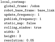
In this case, the local planner uses the frame, since odometry is updated faster and more smoothly than coordinates, which is important for steering control. The reference frame on the robot is, again, the . The local costmap is constructed and updated dynamically based on LIDAR sensing, and thus the parameter is . The local costmap is computed only within a relatively small window about the robot, defined as a with specified dimensions and resolution.
The file is given below:
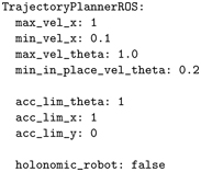
This file sets parameters relevant for steering, including minimum and maximum forward and spin velocities and accelerations. Importantly, since our robot model uses differential drive, it is not holonomic, i.e. it cannot
slip or “crab” sideways. To inform the planner of this, the parameter is set to .
Having defined values for the parameters required for , these parameters should be loaded onto the parameter server for use by . This is accomplished through a launch file. The file in package performs these functions for our example mobile robot. The contents of this file are:
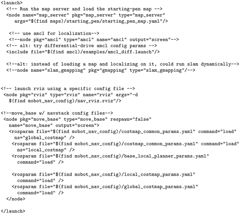
This launch file first loads the starting pen map, then it starts running. In this case, a version of for differential-drive robots is used. (Knowing that the robot cannot slip sideways is helpful in constraining sensor-versus-map localization fits.) is also launched, with reference to a pre-set configuration file. Finally, the node is started, which includes loading the configuration files onto the parameter server for use by . In loading these files, the parameters in are needed by both the global and local planners, and these parameters should be consistent for both. To enforce this consistency, the shared parameters are loaded into the name spaces of the and separately, drawing on the same source file.
Getting good performance from can require considerable tuning of the associated parameters. If these parameters are set inappropriately for a given robot, it can fail to find viable solutions, get stuck at obstacle boundaries, steer erratically, and oscillate at the goal pose.
In addition to tuning the configuration parameters, one has the option of writing a global planner and/or local planner (and steering algorithm) and having these alternative planners operate within (see http://www.w3.org/1999/xlink). One can also use to get to approximate goal poses, then use custom controls to publish to for local precision behaviors (e.g. to approach a charging station approximately with , then perform precision navigation, presumably with sensor feedback, to complete a docking maneuver).
10.3 Example move-base client
The package (with source code ) contains an example of how to construct an action client of the move-base action server. The example can be run by first starting Gazebo with the mobot in the starting pen:

then loading configuration files and starting move-base using :

The example move-base client has a hard-coded goal destination. This is communicated to the move-base action server by running:

This results in generation of a global plan and start of navigation along that plan. Figure 10.9 shows a screenshot of the mobot en route to the goal destination.
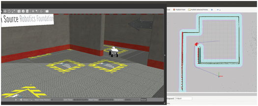
Figure 10.9 Example move-base client interaction. Destination is sent as goal message to move-base action server that plans a route (blue trace) to the destination (triad goal marker).
The example code that sends a navigation goal is shown in Listing 10.1.
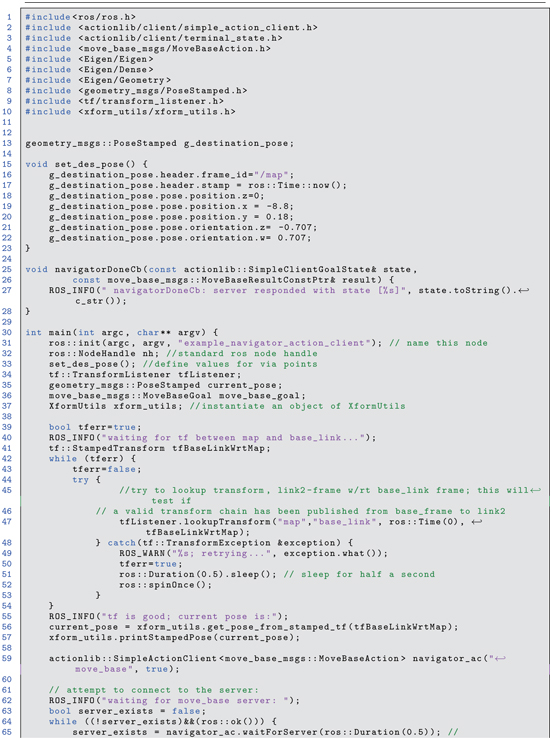
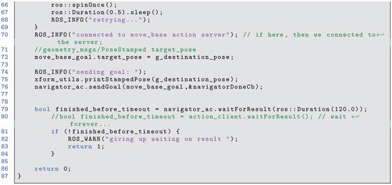
Listing 10.1 example_move_base_client.cpp: example action client of move-base
The move-base action client depends on package , and it includes the corresponding header file (line 4: ). For illustration, a transform listener and the class are also included.
The function merely assigns a hard-coded destination to a object.
Lines 42 through 54 invoke repeated attempts to find the current pose of the robot in the map frame. Once this is successful, the transform is converted to a pose (line 56) and this pose is displayed (line 57).
An action client of is instantiated (line 59), using the action message defined in . The action client attempts to connect to the action server (lines 61 through 70).
A goal message type is instantiated (line 36) and populated with a desired pose (line 72). This goal message is sent to the action server (line 76), and the client then waits for the action server to respond.
By virtue of sending this goal message, the action server plans a global plan from start pose to destination pose, attempting to minimize a cost function that includes penalties for moving too close to obstacles (walls) and a path-length penalty. The resulting global solution is the blue trace in Fig 10.9. The local planner sends velocity commands to the robot to follow local plans that attempt to converge on the global plan while avoiding unexpected obstacles that are perceived along the way.
10.4 Modifying navigation stack
The navigation stack incorporates multiple components, including static and dynamic costmaps, a global planner, and a local planner. The purpose of the local planner is to respond to unexpected obstacles encountered while following the global plan. The default local planner uses a dynamic window approach (see http://www.w3.org/1999/xlink). This reactive planner considers a set of parameterized circular arcs as alternatives to following an invalid global plan (with the intent of re-joining the global plan once the unexpected obstacle is cleared). In this approach, is re-computed during each local-planner controller cycle, which can result in a different arc choice for each iteration. This approach can behave well if the mobile robot does a good job of following each local plan, since iterations of re-planning would then result in reiterating the former (still valid) plan.
However, if the robot does a poor job of following local plans using open-loop velocity commands, the local planner can behave poorly, rejecting its former local plan and substituting a new local plan during each control cycle. In the case of the mobot Gazebo simulation, the robot tends to list to its left. Although this is an artifact of Gazebo’s physics simulation, it is nonetheless a behavior that may be expected in real robots. With a bias error in attempting to execute , the local planner fails to bring the robot back to its original global plan. Consequently, the robot may veer off of a path, fail to successfully drive through navigable narrow passages, or demonstrate poor convergence to goal coordinates.
The local planner can be improved by incorporating a feedback steering algorithm, as discussed in Section 9.3. One way to do this would be to remap the topic of to some other topic, and run a new node that publishes to the robot’s true topic. However, it is convenient to integrate with the considerable resources of , including exploiting the global planner and accessing the costmaps. ROS provides a means to do this by writing and using a plug-in.
A minimal example plug-in that replaces the local planner in is given in the package . This plug-in contains no useful logic; it simply commands the robot to move in a circular arc for 5 sec each time a new navigation goal is specified. The purpose of this example is merely to illustrate the steps to creating a plug-in. (For more details on plug-ins in ROS, see http://www.w3.org/1999/xlink.)
Creating a plug-in requires minor variations on the files and , creation of an additional, small XML file, a specific parameter setting in a corresponding launch file, and application-specific composition of the source files (cpp and header files). These steps are detailed below; composition of the plug-in source code is treated last.
For the minimal example provided, the file follows:
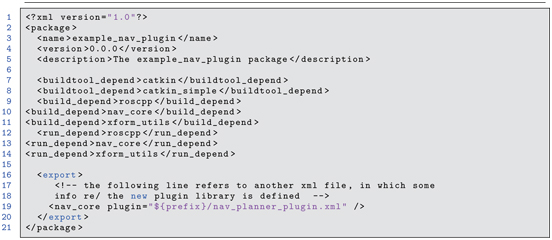
Listing 10.2 package.xml file for example_nav_plugin package
Note the statement on line 19, which specifies the name of an additional XML file (called ). The contents of this additional XML file are:
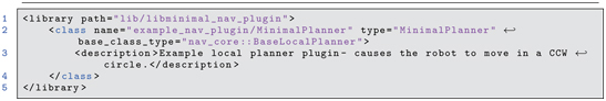
Listing 10.3 nav_planner_plugin.xml
In this additional XML file, one specifies the new library name, the new class name, and the base class from which the new class is derived. In the present case, the name of the library specified in this package’s file is . The compiler will mangle this name to prepend and append and will place the resulting library ( ) in the /devel/lib directory of the ROS workspace.
Within the source code of the new plug-in library, a new class is defined. The source code for this minimal example defines the class . The XML file notes that the definition of is within the package . The XML file also notes that the new class, , is derived from the base class . This is the name of the base class that must be used to replace the local planner. (To replace a global planner, use the base class instead.)
The file within the package contains the line:

This specifies that we are creating a library called . This library will behave as a plug-in, but no further variations are required in the file.
The source code for the plug-in will define a class that, in this example, is called (consistent with the references in ). Assuming the corresponding code has been compiled into the named library ( , in this case), the new plug-in can be used within by setting a corresponding parameter in the launch file. Within the package , the file, specifies how to bring up the navigation stack with use of the new local planner. Only one line of this launch file is different from the default bring-up:

This line specifies that should replace the default with the new class, , from the package .
Finally, we consider the code source files that compose the new plug-in. The header file for our new class, appears in Listing 10.4.
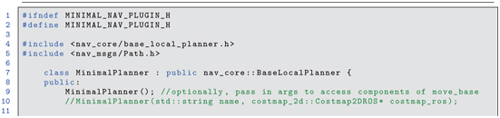
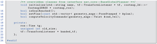
Listing 10.4 minimal_nav_plugin.h
This header file defines the class , which is derived from . The choice of class name must be consistent with the names used in launch file and in the plug-in’s XML file. Four functions are overridden by the new class. The function will get called by the constructor. The function should specify a stopping condition. The function will return if a new global plan has been received, and a reference variable for that plan will provide access to the new plan. Most importantly, the function is responsible for setting the relevant paramters of (forward velocity and yaw rate, in the present case). By setting these values, the node will publish these values as commands to the robot.
The function will be called by at the controller-frequency rate. The rate default is 20 Hz, but this can be changed within the code or by setting a configuration parameter. The current value on the parameter server can be found programmatically with:

The example minimal local planner plug-in source code is relatively short; it is shown in Listing 10.5.
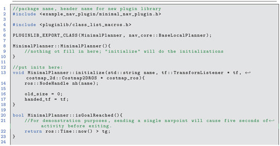
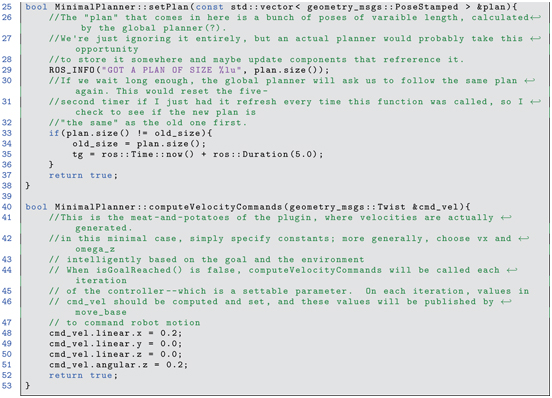
Listing 10.5 minimal_nav_plugin.cpp
A more extensive plug-in example is given in the package of the accompanying repository. This package defines a class with more capability. This alternative plug-in implements a linear steering algorithm, as introduced in Section 9.3.2. It uses the global plan generated by the global planner, from which it computes a time series of desired states. The robot’s pose is inferred from odometry and from AMCL, which localizes the robot relative to a map (of the starting pen, in this example). Linear feedback steering enables the robot to stay on course better, since it compensates for the robot’s tendency to side-slip. The example code in this package also shows how a plug-in can access the nav-stack’s s. This functionality can be used to construct a local planner, such as a “bug” planner that can follow walls, to enable re-connecting with the planned global path.
In addition to overriding the default local planner with a plug-in, one can also write plug-ins for alternative global planners. Additionally, one can create plug-ins for costMaps, which can be useful for annotating features that are not directly accessible to the robot’s sensors. Additional costMap layers can be used, e.g. to impose “no fly” zones for known dangerous areas, such as cliffs or stairwells, glass walls, or terrain that is unnavigable.
10.5 Wrap-Up
The navigation stack is one of the most popular capabilities in ROS. It incorporates consideration of a priori maps, dimensions of the robot, mobility of the robot, and obstacles perceived en route. Subject to constraints on robot speeds and accelerations, a global path plan is constructed from an initial pose to a specified goal pose. Execution of the plan involves a local planner, which takes into consideration perception of nearby obstacles and plans and executes local motions to avoid the obstacles and reconnect with the global plan.
Tuning the parameters of the navigation stack for a specific robot can be time consuming and involves trial and error. Even with these parameters tuned, however, the performance of may be inadequate, particularly if the robot must navigate precisely through narrow passageways (including doorways). It thus may be necessary to interleave goals with custom desired-state generation and steering algorithms to achieve a good balance between generality and precision motion control.
Navigation of the mobot will be revisited in Section VI, in which a combined mobile base and manipulator are integrated to perform mobile manipulation.