Texture Mapping
Texture mapping is a fundamental method for controlling the appearance of rendered objects. A common use of texturing is to provide surface detail to geometry by modifying surface color on a per-pixel basis. A digital image is used as a source of surface color information. Texture mapping can do much more than this, however. It is a powerful and general technique for combining images and geometry. To take advantage of its capabilities, the application designer should understand texturing in depth. This chapter reviews OpenGL’s texture mapping abilities with an emphasis on features important to more complex rendering techniques.
5.1 Loading Texture Images
At the heart of a texture map are the map images, each an n-dimensional array of color values. The individual elements of the array are called texels. The texture image array has one, two, or three dimensions. Core OpenGL requires that the texture image have power-of-two dimensions. The main reason for this is to simplify the computations required to map texture coordinates to addresses of individual texels. This simplification comes at a cost; non-power-of-two sized images need to be padded to a power-of-two size before they can be used as a texture map. There are OpenGL extensions that remove this limit, usually at the expense of some functionality; for example, there is an extension that allows the creation of textures with arbitrary sizes, but restricts the parameter values that can be bound to it, and prohibits mipmapped versions of the texture.1
The glTexImage1D, glTexImage2D, and glTexImage3D commands load a complete texture image, referencing the data in system memory that should be used to create it. These commands copy the texture image data from the application’s address space into texture memory. OpenGL pixel store unpack state describes how the texture image is arranged in memory. Other OpenGL commands update rectangular subregions of an existing texture image (subimage loads). These are useful for dynamically updating an existing texture; in many implementations re-using an existing texture instead of creating a new one can save significant overhead.
The OpenGL pixel transfer pipeline processes the texture image data when texture images are specified. Operations such as color space conversions can be performed during texture image load. If optimized by the OpenGL implementation, the pixel transfer operations can significantly accelerate common image processing operations applied to texture data. Image processing operations are described in Chapter 12.
Texture images are referenced using texture coordinates. The coordinates of a texture map, no matter what the image resolution, range from 0 to 1. Individual texels are referenced by scaling the coordinate values by the texture dimensions. When a texture coordinate is outside the [0, 1] range, OpenGL can be set to wrap the coordinate (use the fractional part of the number), or clamp to the boundaries, based on the value of the texture wrap mode.
5.1.1 Texture Borders
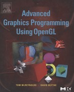
A useful (and sometimes misunderstood) feature of OpenGL is the texture border (Figure 5.1). The border is used by certain wrapping modes to compute texel colors needed by linear filtering when the edge of a texture image is sampled. By definition, the texture border is outside the texture coordinate range of [0, 1]. Texture borders come into play when a texture is sampled near the boundaries of the [0,1] range and the texture wrap mode is set to GL_CLAMP. Textures using GL_NEAREST filtering never sample the border, since this filtering method always uses the nearest texel to the sample point, which is always in the range of [0,1].
When the texture filter is GL_LINEAR, however, texture coordinates near the extremes of 0 or 1 will generate texture colors which are a mix of the border and edge texels of the texture image. This is because linear filtering samples the four texels closest to the sample point. Depending on sample position, up to 3 of these texels may be in the texture border.
The texture border can be specified as a one texel-wide ring of texels surrounding the texture image or as a single color. Individual texels are supplied as part of a slightly bigger texture image; the glTexImage command provides a border parameter to indicate that a border is being supplied. If a border consisting of a single constant color is needed, no border is specified with glTexImage, instead GL_TEXTURE_BORDER_COLOR is specified with the glTexParameter command.
Texture borders are very useful if multiple textures are being tiled together to form a larger one. Without borders, the texture color at the edge of textures using GL_LINEAR filtering would be improperly sampled, forming visible edges. This problem is solved by using edge texels from adjacent textures in the border; each texture is then seamlessly sampling its neighbor’s texels at the edges.
The texture border is one way of ensuring that there are no filtering artifacts at texture boundaries. Another way to avoid filtering artifacts at the tile edges is to use a different clamping mode, called clamp to edge. This mode, added in OpenGL 1.2 and set using the texture parameter GL_CLAMP_TO_EDGE, restricts the sampled texture coordinates so that the texture border is never sampled. The sample is displaced away from the edge so that linear filtering only uses texels that are part of the texture image.
Unlike OpenGL’s standard texture clamping, the clamp to edge behavior is unable to guarantee a consistent border appearance when used with mipmapping, because the clamping range changes with each mipmap level. The clamping range is defined in terms of the texture’s dimensions, which are different at each mipmap level. The clamp to edge behavior is easier to implement in hardware than texture borders because the texture dimensions are not augmented by additional border texels, so the dimensions are always efficient powers of two. As a result, there are OpenGL implementations that support clamp to edge well, but texture border poorly.
5.1.2 Internal Texture Formats
An application can make trade-offs between texel resolution, texture size, and load bandwidth requirements by choosing the appropriate texture format. For example, choosing a GL_LUMINANCE format instead of GL_RGB reduces texture memory usage to one third. A size-specific internal format such as GL_RGBA8 or GL_RGBA4 directs the OpenGL implementation to store the texture with the specified resolution, if it’s supported. The more general internal formats, such as GL_RGBA, leave the implementation free to pick the “most appropriate” format for the particular implementation. If maintaining a particular level of format resolution is important, select a size-specific internal format.
Not all OpenGL implementations support all the available internal texture formats. Requesting GL_LUMINANCE12_ALPHA4, for example, does not guarantee that the texture will be stored in this format. The size-specific internal texture formats are merely hints. The application can exercise more control by querying the OpenGL implementation for supported formats using proxy textures, and picking the most appropriate one.
When choosing lower resolution color formats, some reduction in image quality is unavoidable. Choosing the right trade-off between color resolution and size is not a simple matter. Since textures are applied to particular surfaces, there is more flexibility trading quality for size and load speed than when choosing framebuffer resolutions. For example, a surface texture on an object that will never be close to the viewer, or whose image is composed of similar, low contrast colors, will suffer less if the texture uses a compact texel format. Even texture size is not the dominant issue when and how often the texture will be loaded are also factors to consider. If the texture is static, and its load time doesn’t affect overall performance, then there’s little motivation to improve load bandwidth performance by going to a smaller texel format.
All of these trade-offs are necessarily highly dependent on the details of the application. The best approach is to carefully analyze the use of texture in the application, and use more texel resolution where it has the most impact and the fewest drawbacks. In come cases, re-designing the layout of textures on the objects in the scene makes it possible to get more leverage out of compact texel formats.
5.1.3 Compressed Textures
As another way to reduce the size of texture images, OpenGL includes infrastructure to load texture images using more elaborate compression schemes.2 Reducing the resolution of components can be thought of as one type of compression technique, but other image compression algorithms also exist. The characteristics of a good texture compression algorithm are that it does not reduce the fidelity of an image too much and that individual texels can be easily retrieved from the compressed representation. The glCompressedTexImage commands allow other forms of compressed images to be loaded as texture maps. The core OpenGL specification doesn’t actually define or require any specific compression formats, largely because there isn’t a suitable publicly-available standard format. However, there are some popular vendor-specific formats available as extensions, for example, EXT_texture_compression_s3tc.
5.1.4 Proxy Textures
Texture memory is a limited resource on most graphics hardware; it is possible to run out of it. It is not a trivial task for the application to manage it; the amount of texture memory a particular texture will use is hard to predict and very implementation-dependent. Many graphics applications are also very sensitive to texture load performance; there may be an unacceptable performance penalty if the application simply tries to load the textures that it needs, and executes a recovery scheme when the load fails.
To make it possible for an application to see if a texture will fit before it is loaded, OpenGL provides a proxy texture scheme. The same texture load commands are used, the difference is in the texture target: GL_PROXY_TEXTURE_1D is used in place of GL_TEXTURE_1D, GL_PROXY_TEXTURE_2D in place of GL_TEXTURE_2D, and so on. If these targets are used, the implementation doesn’t load any texture data. Instead it does a “dry run”, indicating to the application whether the texture load would have been successful. This approach may appear awkward, but upon close examination it is actually a superior approach. It works well because of its flexibility; it can accurately report back whether space is available for the texture specified regardless of the number of texture loads that have already happened, what internal texture format the OpenGL implementation has chosen, or details of the underlying graphics hardware.
If the load would not have succeeded, OpenGL doesn’t signal an error, but instead sets all the texture state to zero. The application can read back any element of this state to determine the success of the load request. A simple way to check for success is to call glGetTexLevelParameter, again using the proxy texture target, the appropriate level, and a state parameter that shouldn’t be zero, such as GL_TEXTURE_WIDTH. If the width is zero, the texture load would have failed.
Determining whether there is space for a full mipmap array requires a subtle change. Rather than loading the base image level, normally zero, a level greater than the base level is loaded. This indicates to the proxy mechanism whether to calculate space for just the base level or to compute it for the entire array, starting from the base level and ending at the maximum array level.
Proxy texture requests don’t simply check for available space; they check the entire texture state. A proxy texture command will fail if an invalid state is specified, even if there is enough room for the texture. However, this type of failure shouldn’t occur for debugged production programs.
5.2 Texture Coordinates
Texture coordinates associate positions on the texture image to the textured primitive’s vertices. The per-vertex assignment of texture coordinates provide an overall mapping of a texture image to rendered geometry. During rasterization, the texture coordinates of a primitive’s vertices are interpolated over the primitive, assigning each rasterized fragment its own texture coordinates.
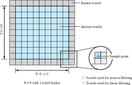
In OpenGL, a vertex of any primitive (and the raster position of pixel images) can have texture coordinates associated with it. Figure 5.2 shows how a primitive’s position and texture coordinate values at each vertex establish a relationship between a texture image and the primitive.
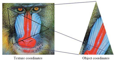
Figure 5.2 Vertices with texture coordinates. Texture coordinates determine how a texture maps to the triangle.
OpenGL generalizes the notion of a two-component texture coordinate (s,t) into a four-component homogeneous texture coordinate (s,t,r,q). The q coordinate is analogous to the w component found in vertex coordinates, making texture coordinates homogeneous. Homogeneous coordinates make correct texturing possible even if the texture coordinates are perspectively projected. The r coordinate allows for 3D texturing in implementations that support it.3 The r coordinate is interpolated in a manner similar to s and t. OpenGL provides default values for both r (0) and q (1).
A primitive being rasterized may have w values that aren’t unity. This commonly occurs when the projection matrix is loaded with a perspective projection. To apply a texture map on such a primitive without perspective artifacts, the texture coordinates must be interpolated with a method that works correctly with perspective projection. A well-known method is to divide the texture coordinates at each vertex by the vertex’s w component, interpolate the resulting values for each fragment, then divide the resulting values by a 1/w component that has also been interpolated from 1/w values computed at the vertices (Blinn, 1992). For a more detailed discussion of perspective correct vertex interpolation see Section 6.1.4.
Since OpenGL supports a texture transform matrix, the texture coordinates themselves can be projected through a perspective transform. To avoid artifacts created by projected texture coordinates, the texture values should also be scaled by the interpolated q value. So rather than interpolating (s/w,t/w,r/w) at each fragment, then dividing by 1/w, the division step becomes a division by q/w, where q/w is also interpolated to the fragment position. Thus, in implementations that perform perspective correction, there is no extra rasterization burden associated with processing q (Segal and Akeley, 2003).
OpenGL can apply a general 4×4 transformation matrix followed by a perspective divide to texture coordinates before using them to apply the texture map. This transform capability allows textures to be rotated, scaled, and translated on the geometry. It also allows texture coordinates to be projected onto an arbitrary plane before being used to map texture to geometry. Although the texture pipeline only has a single transform matrix compared to the geometry pipeline’s two, the distinction can still be made between modelview and projective transforms. The difference is now conceptual, however, since all transforms must share a single matrix.
5.2.1 Texture Coordinate Generation and Transformation
An alternative to assigning texture coordinates explicitly is to have OpenGL generate them. OpenGL texture coordinate generation (called texgen for short) generates texture coordinates from other components in the vertex. Sources include position, normal vector, or reflection vector (computed from the texture position and its normal). Texture coordinates computed from vertex positions are created from a linear function of eye-space or object-space coordinates. Texture coordinates computed from reflection vectors can have three components, or be two-component coordinates produced from a projection formula.
OpenGL provides a 4×4 texture matrix used to transform the texture coordinates, whether supplied explicitly with each vertex, or implicitly through texture coordinate generation. The texture matrix provides a means to rescale, translate, or even project texture coordinates before the texture is applied during rasterization.
Figure 5.3 shows where texture coordinates are generated in the transformation pipeline and how they are processed by the texture transform matrix. Only GL_OBJECT_LINEAR and GL_EYE_LINEAR modes are shown here. Note that the texture transformation matrix transforms the results, just like it does if texture coordinates are sent explicitly.
5.3 Loading Texture Images from the Frame Buffer
Texture map images are created by storing bitmaps into a texture. The direct approach is for the application to supply the image, then load it with glTexImage2D. A less obvious but powerful approach is to create the texture dynamically instead; rendering an image into the framebuffer, then copying it into a texture. Transferring an image from the color buffer to a texture is a simple procedure in OpenGL. The image is rendered, then the resulting image is read back into system memory buffer using glReadPixels. The application can then use the buffer to load a texture with glTexImage2D.
In later versions of OpenGL,4 the process was streamlined. A region of a framebuffer image can now be copied directly into a texture using glCopyTexImage, bypassing the glReadPixels step and improving performance. This technique is so useful that aWGL extension, ARB_render_texture, makes the method even more efficient. It does away with the copy step entirely, making it possible to render an image directly into a texture. The new feature is not an extension of core OpenGL. It is an extension of the OpenGL embedding layer (described in Chapter 7), adding the ability to configure a texture map as a rendering target. OpenGL can be used to render to it, just as if it was a color buffer. See Section 14.1 for more information on transferring images between textures and framebuffers, and how it can be a useful building block for graphics techniques.
5.4 Environment Mapping
Scene realism can be improved by modeling the lighting effects that result from inter-object reflections. OpenGL provides an ambient light term in its lighting equation, but this is only the crudest approximation to the lighting environment that results from light reflecting off of other objects. A more sophisticated approach is available through the use of OpenGL texturing functionality. The term environment mapping describes a texturing technique used to model some of the influences of the surrounding environment on an object’s appearance.
Environment mapping, like regular surface texturing, changes an object’s appearance by applying a texture map to its surface. An environment texture map, however, takes into account the surrounding view of the object’s environment. If the object’s surface has high specularity, the texture map shows surrounding objects reflected off of the surface. Objects with low specularity can be textured with an image approximating the radiance coming from the surrounding environment.
The environment map, once created, must be properly applied to an object’s surface. Since it is simulating a lighting effect, texels are selected as a function of the normal vector or reflection vector at each point on the surface. These vectors are converted into texture coordinates at each vertex, then interpolated to each point on the surface, as they would for a regular surface texture. Using these vectors as inputs to the texture generation function makes it possible to simulate the behavior of diffuse and specular lighting artifacts.
5.4.1 Generating Environment Map Texture Coordinates
The OpenGL environment mapping functionality is divided into two parts: a set of texture coordinate generation functions, and an additional texture map type called a cube map. To maximize flexibility, the two groups are orthogonal; texture generation functions can be used with any type of texture map, and cube map textures can be indexed normally with three texture coordinates. There are three texture generation functions designed for environment mapping; normal mapping, reflection vector mapping, and sphere mapping. A function can be selected by setting the appropriate parameter to glTexGen command: GL_NORMAL_MAP, GL_REFLECTION_MAP, or GL_SPHERE_MAP.
Normal vector texture generation makes it possible to apply a texture map onto a surface based on the direction of the surface normals. It uses the three component vertex normals as texture coordinates, mapping Nx, Ny, and Nz into s, t, and r, respectively. Normal vectors are assumed to be unit length, so the generated texture coordinates range from −1 to 1. This technique is useful for environment mapping an object’s diffuse reflections; the surface color becomes a function of the surface’s orientation relative to the light sources of its surroundings.
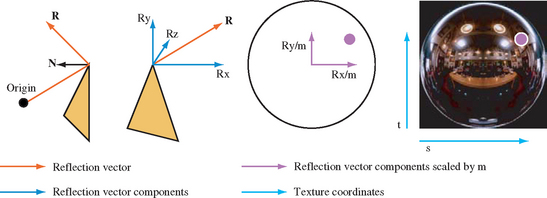
Reflection texture generation indexes a surface texture based on the component values of the reflection vector. The reflection vector is computed using the vertex normal and an eye vector. The eye vector is of unit length, pointing from the eye position toward the vertex. Both the eye vector U, and the reflection vector R, are computed in eye space. The reflection vector is generated by applying the equation R = U − 2NT(U · N), where N is the vertex normal transformed into eye space. The reflection equation used is the standard for computing the reflection vector given a surface normal and incident vector.5
Once the reflection vector is computed, its components are converted to texture coordinates, mapping Rx, Ry, and Rz to s, t, and r, respectively. Because N and U are normalized, the resulting R is normalized as well, so the texture coordinates will range from −1 to 1. This function is useful for modeling specular objects, whose lighting depends on both object and viewer position.
Sphere map texture generation has been supported by OpenGL since version 1.0. While the other two texture generation modes create three texture coordinates, sphere map generation only produces two; s and t. It does this by generating a reflection vector, as defined previously, then scaling the Rx and Ry components by a modified reflection vector length, called m. The m length is computed as ![]() . Dividing the Rx and Ry by this m length projects the two components into a vector describing a unit circle in the Rz = 0 plane. When these scaled Rx and Ry vectors are scaled by
. Dividing the Rx and Ry by this m length projects the two components into a vector describing a unit circle in the Rz = 0 plane. When these scaled Rx and Ry vectors are scaled by ![]() and biased by
and biased by ![]() , they are bounded to a [0,1] range and can be used as s and t coordinates. While the other texture generation modes create three texture coordinates, requiring a texture map that can index them (usually a cube map), the sphere map generation function can be used with a normal 2D texture (Figure 5.4).
, they are bounded to a [0,1] range and can be used as s and t coordinates. While the other texture generation modes create three texture coordinates, requiring a texture map that can index them (usually a cube map), the sphere map generation function can be used with a normal 2D texture (Figure 5.4).
5.4.2 Texture Maps Used in Environment Mapping
The following sections describe the two basic OpenGL environment mapping techniques: sphere mapping and cube mapping (for a description of another environment mapping method, dual paraboloid mapping, see Section 14.8).
We’ll consider the creation and application of environment textures, as well as the limitations associated with their usage. In both cases, sampling issues are paramount. Any functionality that converts normal vectors into texture coordinates will have sampling issues. Since texture maps themselves are not spherical, any coordinate generation method will produce sampling rates that vary across the texture. Another important consideration when evaluating environment maps is the effort required to create an environment map texture. This issue looms larger when environment maps must be created dynamically, or if the environment mapping technique is not view-independent.
5.4.3 Cube Mapping
From its first specification, OpenGL supported environment mapping, but only through sphere map texture generation. With OpenGL 1.3, cube map textures, partnered with normal and reflection texture coordinate generation, have been added to augment OpenGL’s environment mapping capabilities. A cube map texture is composed of six 2D texture maps, which can be thought of as covering the six faces of an axis-aligned cube. The s, t, and r texture coordinates form the components of a normalized vector emanating from the cube’s center. Each component of the vector is bound to the range [−1, 1]. The vector’s major axis, the axis of the vector’s largest magnitude component, is used to select the texture map (cube face). The remaining two components index the texels used for filtering. Since the components range from −1 to 1, the filtering step scales and biases the values into the normal 0 to 1 range so they can be used to index into the cube face’s 2D texture.
Cube map functionality has been added to the OpenGL in a very orthogonal manner, so the OpenGL commands and methodology needed to use them should be familiar. To use a cube map, the cube map textures must be loaded, configured, and enabled. The appropriate texture coordinates must be set or generated (the latter is the more common case) for each vertex. A cube map texture can be loaded with the usual OpenGL functions, including glTexImage2D and glCopyTexImage2D. The target must be set to one of the six cube map faces, listed in Table 5.1.
Table 5.1
The OpenGL enumeration values are consecutive, and increase from the top to the bottom of the table. This enumerant ordering makes it easier to load the images using a loop construct in the application code. Cube map texturing is enabled using glEnable with an argument of GL_TEXTURE_CUBE_MAP.
Each cube map face can be a single 2D texture level or a mipmap. The usual procedures apply; the only difference is in the texture target name. The appropriate texture target shown in Table 5.1 must be used in the place of GL_TEXTURE_2D. The same caveats and limitations also apply; if the cube map does not have mipmapped faces, its minification filter must be set to an appropriate type, such as GL_LINEAR. The minification filter of GL_LINEAR_MIPMAP_LINEAR is the default minification value, just as it is for 2D textures.
If the application enables multiple texture maps at the same time, cube map textures take precedence over 1D, 2D, or 3D texture maps. If multitexturing is used, cube map textures can be bound to one or more texture units. Multiple cube maps can also be managed with texture objects.
As noted previously, a cube map can be indexed directly using texture coordinates. A 3D set of texture coordinates must be applied to each vertex, using a command such as glTexCoord3f. Although setting texture coordinates directly can be useful, especially for debugging, the most common way to index cube map textures is with a texture generation function. In this case, the texture generation function should create s, t, and r components. To set the s coordinate to reflection texture generation, the glTexGen function is set with the GL_S coordinate, the GL_TEXTURE_GEN_MODE parameter, and the GL_REFLECTION_MAP value.
The combination of a texture generation function and a cube map can be thought of as a programmable function that can take as input one of two types of 3D vectors.; the texture map provides the filtered table lookup, while the texture coordinate generation provides the input vector. The GL_EYE_LINEAR texgen provides the eye vector to the vertex, GL_NORMAL_MAP provides the vertex’s normal, and GL_REFLECTION_MAP provides its reflection vector.
Cube Map Texture Limitations
Although very powerful, cube map texturing has a number of important limitations. Since the textures aren’t spherical, the sampling rate varies across each texture face. The sample rate is best at the center of each texture face; a fixed angular change in direction cuts through the smallest number of texels at this point. The ratio between the best and worst sampling rates is signficant; although better than sphere maps, it is worse than dual paraboloid maps.
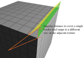
Sampling across cube face boundaries can also be an issue. Since a cube texture is composed of six non-overlapping pieces, creating textures that provide good border sampling isn’t trivial. Cube map textures with borders must correctly sample texel values from their neighbors; because of the cube geometry, simply using a strip of texels from adjacent textures will result in slightly inaccurate sampling. The border texels must be projected back along the line to the cube center to find the adjacent cube samples that provide their colors.
Things get more complex if mipmapped textures with borders are used. Border texels cover different areas, depending on the coarseness of the mipmap level. Mipmap textures with borders handle texture coordinates generated from rapidly changing vertex vectors. An example is a small triangle, covering only a few pixels on the screen, containing three highly divergent vertex normals. Normal or reflection vector interpolation leads to adjacent pixels sampled from different faces of the cube map; only good texture generation will avoid aliasing artifacts in these conditions.
If a geometry primitive with antiparallel vectors is interpolated, the interpolated vector may become degenerate. In this case, the sampled texel will be arbitrary. A cube map with mipmapped face textures will reduce the chance of aliasing in this case. Such interpolations have a large derivative value, and the coarse mipmap levels of the cube faces tend to have similar texel colors. Cube map textures also consume lots of texture memory. For any given texture resolution (which because of the sampling rate variations, tend to be large to maintain quality), the texture memory usage must be multipled by six to take into account all of the cube faces.
5.4.4 Sphere Mapping
Sphere mapping is the original environment mapping method for OpenGL; it has been a core feature since OpenGL 1.0. A sphere map texture is a normal 2D texture with a specially distorted image on it. The sphere map image is inscribed in the interior of a circle in the texture map with radius ![]() centered at (
centered at (![]() ,
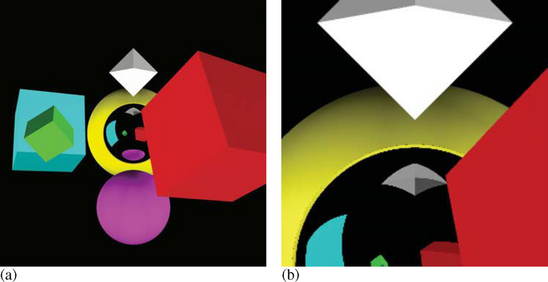
, ![]() ) in texture coordinates. The image within the circle can be visualized as the image of a chrome sphere reflecting its surroundings. The silhouette edge of the sphere is seen as an extreme grazing reflection of whatever is directly behind the sphere. Visualize the sphere as infinitely small; it doesn’t obscure any objects, and its grazing reflection is of only one point behind it. This implies that, ignoring sampling issues, every point on the circle’s edge of a properly generated sphere map should be the same color. Properly normalized reflection vectors are guaranteed to fall within the sphere map’s circle, so texels outside the circle will never be filtered.
) in texture coordinates. The image within the circle can be visualized as the image of a chrome sphere reflecting its surroundings. The silhouette edge of the sphere is seen as an extreme grazing reflection of whatever is directly behind the sphere. Visualize the sphere as infinitely small; it doesn’t obscure any objects, and its grazing reflection is of only one point behind it. This implies that, ignoring sampling issues, every point on the circle’s edge of a properly generated sphere map should be the same color. Properly normalized reflection vectors are guaranteed to fall within the sphere map’s circle, so texels outside the circle will never be filtered.
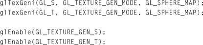
Since sphere mapping requires only a single texture, configuring OpenGL for sphere mapping is straightforward. The desired sphere map texture is made current, then texturing is done in the usual manner. The sphere map texture image is designed to map texture coordinates derived from reflection vectors at each vertex. Although regular texture coordinates can be used, OpenGL provides a special texture coordinate generation mode that can be used to map texture coordinates from reflection vectors. Since a sphere map texture is 2D, only the s and t coordinates need to be generated:
As with any environment mapping technique, the combination of sphere map texture and sphere map texture coordinate generation can be thought of as a 2D mapping function converting reflection vector directions into color values.
Sphere Map Limitations
Although sphere mapping can be used to create convincing environment mapped objects, sphere-mapped reflections are not physically correct. Most of the artifacts come from the discrepancy between a sphere map image generation and its application onto textured geometry. A sphere map image is mapped as if its reflection vectors originate from a single location. On the other hand, a sphere map texture is often applied over the extended area of an object’s surface. As a result, sphere-mapped objects can’t accurately reproduce the optical effect of reflecting a nearby object, or represent a reflective object that is self-reflecting. Sphere mapping results are only completely accurate when the assumption is made that all of the reflected surroundings are infinitely far from the reflective object.
The variable sampling rate of sphere map can also lead to sampling artifacts. The computed texture coordinates are perspective correct at the vertices, but linearly interpolated across each polygon. Unfortunately, a sphere map image is highly non-linear, so this interpolation is not correct. This can lead to poor sampling rates for the parts of the textured primitive that sample near the edge of the sphere map circle, with the usual aliasing artifacts.
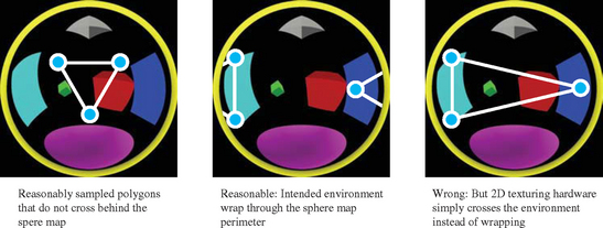
Additionally, the points at the edge of the sphere-map circle all map to the same location. This can lead to multiple valid but varying interpolations for the same set of vertex texture coordinates; interpolating within the sphere map circle, or interpolating the “long way around,” across the sphere-map circle boundary. This type of interpolation is necessary when the reflecting primitive is nearly edge on to the viewer. In these cases, sphere map coordinates will be interpolated incorrectly, since they always interpolate within the sphere map circle. Figure 5.6 illustrates this ambiguity.
The failure to wrap around the sphere map edge is responsible for an unsightly artifact that appears as random “sparkles” or “dirt” at the silhouette edge of a sphere-mapped object. The wrong texels are used to texture the polygons, causing the object to have miscolored regions. Generally the incorrectly sampled polygons are small, causing the artifacts to look like “dirt”. Because these grazing polygons are small in screen space, the number of affected pixels is usually small. Still the effectively random sparkling can be objectionable, particularly in animated scenes. Figure 5.7 shows a scene with sparkle artifacts, a zoomed in section of the scene sparkles at the silhouette edge of the sphere-mapped object.
This problem can be solved by careful splitting of silhouette polygons, forcing the correct texels to be sampled in the resulting polygons. The polygons should be split along the boundary of the polygon where the interpolated reflection vector is parallel to the direction of view (and maps to the the sphere map edge). This can be an expensive operation, however. It may be better to use a more robust technique such as cube mapping.
The final major limitation of sphere maps is that their construction assumes that the center of the sphere map reflects directly back at the viewer. When constructing sphere maps, the construction is based on a particular view orientation. The sphere map image is view-dependent. This means unless the sphere map is regenerated for different views, the sphere map will be incorrect as the viewer’s relationship to the textured object changes.
To avoid artifacts, new sphere map texture images must be created and loaded as the viewer/object relationship changes. If the environment mapped object is reflecting a dynamic environment, this continuous updating may be required anyway. This requirement is a major limitation for using sphere maps in dynamic scenes with a moving viewer.
5.5 3D Texture
An important point to note about 3D textures in OpenGL is how similar they are to their 1D and 2D relatives. From the beginning, OpenGL texturing was designed to be extensible. As a result, 3D textures are implemented as a straightforward extension of 2D and 1D textures. Texture command parameters are similar; a GL_TEXTURE_3D target is used in place of GL_TEXTURE_2D or GL_TEXTURE_1D.6 The texture environment remains unchanged. 3D texture internal and external formats and types are the same, although a particular OpenGL implementation may limit the availability of 3D texture formats.
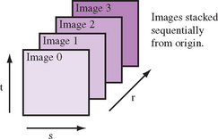
A 3D texture is indexed with s, t, and r texture coordinates instead of just s and t. The additional texture coordinate complexity, combined with the common uses for 3D textures, means texture coordinate generation is used more commonly for 3D textures than for 1D and 2D. Figure 5.8 shows a 3D texture, its 2D image components, and how it is indexed with s, t, and r.
3D texture maps take up a large amount of texture memory, and are expensive to change dynamically. This can affect the performance of multipass algorithms that require multiple passes with different textures.
The texture matrix operates on 3D texture coordinates in the same way that it does for 1D and 2D textures. A 3D texture volume can be translated, rotated, scaled, or have any other combination of affine and perspective transforms applied to it. Applying a transformation to the texture matrix is a convenient and high-performance way to manipulate a 3D texture, especially when it is too expensive to alter the texel values directly.
A clear distinction should be made between 3D textures and mipmapped 2D textures. 3D textures can be thought of as a solid block of texture, requiring a third texture coordinate r, to access any given texel. A 2D mipmap is a series of 2D texture maps, each filtered to a different resolution. Texels from the appropriate level(s) are chosen and filtered, based on the relationship between texel and pixel size on the primitive being textured.
Like 2D textures, 3D texture maps may be mipmapped. Instead of resampling a 2D image, at each level the entire texture volume is resampled down to an eighth of its volume. This is done by averaging a group of eight adjacent texels on one level down to a single texel on the next. Mipmapping serves the same purpose in both 2D and 3D texture maps; it provides a means of accurately filtering when the projected texel size is small relative to the pixels being rendered.
5.5.1 Using 3D Textures to Render Solid Materials
A straightforward 3D texture application renders solid objects composed of heterogeneous material. A good example would be rendering an object made of solid marble or wood. The object itself is composed of polygons or non-uniform rational B-splines (NURBS) surfaces bounding the solid. Combined with proper texgen values, rendering the surface using a 3D texture of the material makes the object appear cut out of the material. In contrast, with 2D textures, objects often appear to have the material laminated on the surface. The difference can be striking when there are obvious 3D coherencies in the material texture, especially if the object has sharp angles between its surfaces.
Creating a solid 3D texture starts with material data. The material color data is organized as a three dimensional array. If mipmap filtering is desired, use glBuild3DMipmaps to create the mipmap levels. Since 3D textures can use up a lot of texture memory, many implementations limit their maximum allowed size. Verify that the size of the texture to be created is supported by the system and there is sufficient texture memory available for it by calling glTexImage3D with GL_PROXY_TEXTURE_3D to find a supported size. Alternatively, glGet with GL_MAX_3D_TEXTURE_SIZE retrieves the maximum allowed size of any dimension in a 3D texture for the OpenGL implementation, though the result may be more conservative than the result of a proxy query, and doesn’t take into account the amount of available texture memory.
The key to applying a solid texture accurately on the surface is using the right texture coordinates at the vertices. For a solid surface, using glTexGen to create the texture coordinates is the easiest approach. Define planes for s, t, and r in object space to orient the solid material to the object. Adjusting the scale has more effect on texture quality than the position and orientation of the planes, since scaling affects the spacing of the texture samples.
Texturing itself is straightforward. Using glEnable(GL_TEXTURE_3D) to enable 3D texture mapping and setting the texture parameters and texture environment appropriately is all that is required. Once properly configured, rendering with a 3D texture is no different than other types of texturing. See Section 14.1 for more information on using 3D textures.
5.6 Filtering
While texture image is a discrete array of texels, texture coordinates vary continuously (at least conceptually) as they are interpolated across textured primitives during rendering. This creates a sampling problem. When rendering textured geometry, the difference between texture and geometric coordinates causes a pixel fragment to cover an arbitrary region of the texture image (called the pixel footprint). Ideally, texture filtering integrates weighted contributions from all the texels covered by the pixel footprint. The discussions in Section 4.1 regarding digital image representation and sampling are equally valid when applied to texture mapping. Texture mapping operations can introduce aliasing artifacts if inadequate sampling is performed. In practice, texture mapping doesn’t approach ideal sampling because of the large performance penalty incurred by accessing and integrating all contributing sample values. In some circumstances, filtering results can be improved using special techniques inside the application. For example, Section 14.7 describes techniques for dealing with anisotropic footprints.
OpenGL provides a set of filtering methods for sampling and integrating texel values. The available filtering choices depend on whether the texels are being magnified (when the pixel footprint is smaller than a single texel) or minified (the pixel footprint is larger than a single texel).
The simplest filter method is point sampling: only a single texel value, from the texel nearest the texture coordinate’s sample point, is selected. This type of sampling, called GL_NEAREST in OpenGL, is useful when an application requires access to unmodified texel values (e.g., when a texture map is being used as a lookup table). Point sampling seldom gives satisfactory results when used to add surface detail, often creating distracting aliasing artifacts. Instead, most applications use an interpolating filter.
Bilinear texturing is the next step up for filtering texture images. It performs a linear interpolation of the four texels closest to the sample point. In image processing parlance, this is a tent or triangle filter using a 2×2 filter kernel. In OpenGL this type of filtering is referred to as GL_LINEAR. For magnified textures, OpenGL supports GL_LINEAR and GL_NEAREST filtering. For minification, OpenGL supports GL_NEAREST and GL_LINEAR, as well as a number of different mipmapping (Williams, 1983) approaches. The highest quality (and most computationally expensive) mipmap method core OpenGL supports is tri-linear mipmapping. This mipmapping method, called GL_LINEAR_MIPMAP_LINEAR, performs bilinear filtering on the two closest mipmap levels, then interpolates the resulting values based on the sample point’s level of detail.
Some OpenGL implementations support an extension called SGIS_texture_filter4. This is a texture filtering method that provides a larger filter kernel. It computes the weighted sum of the 4×4 texel array closest to the sample point. Anisotropic texturing, which handles textures with a higher minification value in a certain direction (this is common in textures applied to geometry that is viewed nearly edge on), is also supported by some OpenGL implementations with the EXT_texture_filter_anisotropic extension. Anisotropic texturing samples a texture along the line of maximum minification. The number of samples depends on the ratio between the maximum and minimum minification at that location.
5.7 Additional Control of Texture Level of Detail
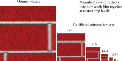
In OpenGL 1.0 and 1.1, all of the mipmap levels of a texture must be specified and consistent. To be consistent, every mipmap level of a texture must have half the dimensions of the previous mipmap level of detail (LOD) until reaching a level having one or both dimensions of length one, excluding border texels. In addition, all of a mipmap’s levels must use the same internal format and border configuration (Figure 5.9).
If mipmap filtering is requested for a texture, but all the mipmap levels of a texture are not present or are not consistent, OpenGL silently disables texturing. A common pitfall for OpenGL programmers is to accidently supply an inconsistent or incomplete set of mipmap levels, resulting in polygons being rendered without texturing. For a common example of this problem, consider an application that specifies a single texture level without setting the minification filter setting. The default minification filter in OpenGL, GL_LINEAR_MIPMAP_LINEAR, requires a consistent mipmap. As a result, the texture is inconsistent with the minification filter being used, and texturing is disabled.
OpenGL 1.2 relaxes the texture consistency requirement by allowing the application to specify a contiguous subset of mipmap levels to use. Only the levels specified must exist and be consistent. For example, this feature permits an application to specify only the 1×1 through 256×256 mipmap levels of a texture with a 1024×1024 level 0 texture, and still mipmap with these levels, even if the 512×512 and 1024×1024 levels are not loaded. The application can do this by setting the texture’s GL_TEXTURE_BASE_LEVEL and GL_TEXTURE_MAX_LEVEL parameters appropriately. An OpenGL application will not use texture levels outside the range specified by these values, even if the level of detail parameter indicates that they are the most appropriate ones to use.
The level of detail parameter, λ, is used in the OpenGL specification to describe the size relationship between a pixel in window space, and the corresponding texel(s) that covers it. If the texture coordinates of a textured primitive were overlayed onto the primitive in screen space, and the texture coordinates were scaled by the texture dimensions, the ratio of these coordinates shows how the texels in the texture map correspond to the pixels in the primitive. A ratio can be computed for each texture coordinate relative to the x and y coordinates in window space. Taking log2 of the largest scale factor produces λ. This parameter is measured to choose between minification and magnification filters, and to select mipmap levels when mipmap minification is enabled.
Limiting OpenGL to a limited range of texture levels is useful if an application must guarantee a constant update rate. From the previous example, if texture load bandwidth is a bottleneck, the application might constrain the base and maximum LODs when it doesn’t have enough time to load the 512×512 and 1024×1024 mipmap levels from disk. In this case, the application chooses to settle for lower resolution LODs, possibly resulting in blurry textured surfaces, rather than not updating the image in time for the next frame. On subsequent frames, when the application gets enough additional time to load the full set of mipmap levels for the texture, it can load the finer levels, change the LOD limits, and render with full texture quality. The OpenGL implementation can be configured to use only the available levels by clamping the λ LOD value to the range of available ones.
OpenGL provides finer control over LOD than specifying a range of texture levels. The minimum and maximum allowable LOD values themselves can be specified. The OpenGL 1.2 GL_TEXTURE_MIN_LOD and GL_TEXTURE_MAX_LOD texture parameters provide a further means to clamp the λ LOD value. The min and max values can be fractional, allowing the application to control the blending of two mipmap levels.7 An application can use the min and max values to gradually “sharpen up” to a finer mipmap level over a number of frames, or gradually “blur down” to a coarser level.
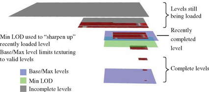
This functionality can be used to make the use of finer texture levels as they become available less abrupt and noticeable to the user. Section 14.6 applies this feature to the task of texture paging. Figure 5.10 shows how texture level and LOD ranges can work together to allow the application fine control over loading and using a mipmap. In this example, a mipmap’s levels are being loaded over a number of frames. LOD control is used to ensure that the mipmap can be put to use while the loading occurs, with minimal visual artifacts.
5.8 Texture Objects
Most texture mapping applications switch among many different textures during the course of rendering a scene. To facilitate efficient switching among multiple textures and to facilitate texture management, OpenGL uses texture objects to maintain texture state.8
The state of a texture object contains all of the texture images in the texture (including all mipmap levels) and the values of the texturing parameters that control how texels are accessed and filtered. Other OpenGL texture-related states, such as the texture environment or texture coordinate generation modes, are not part of a texture object’s state.
As with display lists, each texture object is identified by a 32-bit unsigned integer which serves as the texture’s name. Like display list names, the application is free to assign arbitrary unused names to new texture objects. The command glGenTextures assists in the assignment of texture object names by returning a set of names guaranteed to be unused. A texture object is bound, prioritized, checked for residency, and deleted by its name. Each texture object has its own texture target type. The four supported texture targets are:
The value zero is reserved to name the default texture of each texture target type. Calling glBindTexture binds the named texture object, making it the current texture for the specified texture target. Instead of always creating a new texture object, glBindTexture creates a texture object only when a texture image or parameter is set to an unused texture object name. Once created, a texture object’s target (1D, 2D, or 3D) can’t be changed. Instead, the old object must be destroyed and a new one created.
The glTexImage, glTexParameter, glGetTexParameter, glGetTexLevelParameter, and glGetTexImage commands update or query the state of the currently bound texture of the specified target type. Note that there are really four current textures, one for each texture target type: 1D, 2D, 3D, and cube map. When texturing is enabled, the current texture object (i.e., current for the highest priority enabled texture target) is used for texturing. When rendering geometric objects using more than one texture, glBindTexture can be used to switch among them.
Switching textures is a fairly expensive operation; if a texture is not already resident in the accelerator texture memory, switching to a non-resident texture requires that the texture be loaded into the hardware before use. Even if the texture is already loaded, caches that maximize texture performance may be invalidated when switching textures. The details of switching a texture vary with different OpenGL implementations, but it’s safe to assume that an OpenGL implementation is optimized to maximize texturing performance for the currently bound texture, and that switching textures should be minimized.
Applications often derive significant performance gains sorting the objects they are about to render by texture. The goal is to minimize the number of glBindTexture commands required to draw the scene. Take a simple example: if a scene uses three different tree textures to draw several dozen trees within a scene, it is a good idea to group the trees by the texture they use. Then each group can be rendered in turn, binding the group’s texture, then rendering all the group’s members.
5.9 Multitexture
OpenGL 1.3 extends core texture mapping capability by providing a framework to support multiple texture units. This allows two or more distinct textures to be applied to a fragment in one texturing pass.9 This capability is generally referred to by the name multitexture. Each texture unit has the ability to access, filter, and supply its own texture color to each rasterized fragment. Before multitexture, OpenGL only supported a single texture unit. OpenGL’s multitexture support requires that every texture unit be fully functional and maintain state that is independent of all other texture units. Each texture unit has its own texture coordinate generation state, texture matrix state, texture enable state, and texture environment state. However, each texture unit within an OpenGL context shares the same set of texture objects.
Rendering algorithms that require multiple rendering passes can often be reimplemented to use multitexture and operate with fewer passes. Some effects, due to the number of passes required or the need for high color precision, are only viable using multitexture.
Many games, such as Quake (id Software, 1999) and Unreal (Epic Games, 1999), use light maps to improve the lighting quality within their scenes. Without multitexture, light map textures must be modulated into the scene using a second blended rendering pass, after the first pass renders the surface texture. With multitexture, the light maps and surface texture can be rendered in a single rendering pass. This reduces the transformation overhead almost in half: rendering light maps as part of a single multitextured rendering pass means the polygons are only transformed once. Framebuffer update overhead is also lower when using multitexture to render light maps: when multitexture is used, the overhead of blending in the second rendering pass is eliminated. The computation moves from the framebuffer blending part of the pipeline to the second texture unit’s environment stage. This means the light maps only affect the processing of multitextured geometry, rather than the entire scene. Light maps are described in more detail in Section 15.5.
5.9.1 Multitexture Model
The multitexture API adds commands that control the state of one or more texture units. The glActiveTexture command determines which texture unit will be affected by the OpenGL texture commands that follow. For example, to enable 2D texturing on texture unit 0 and 1D texturing on texture unit 1, issue the following OpenGL commands:
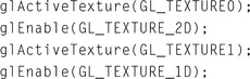
Note that the state of each texture unit is completely independent. When multitexture is supported, other texture commands such as glTexGen, glTexImage2D, and glTexParameter affect the current active texture unit (as set by glActiveTexture). Other commands, such as glDisable, glGetIntegerv, glMatrixMode, glPushMatrix, and glPopMatrix, also operate on the current active texture unit when updating or querying texture state.
The number of texture units available in a given OpenGL implementation can be found by querying the implementation-dependent constant GL_MAX_TEXTURE_UNITS. using glGetIntegerv. To be conformant with the OpenGL specification, implementations should support at least two units, but this may not always be the case. To be safe, the application should query the number available before multitexturing.
OpenGL originally supported a single set of texture coordinates. With the addition of multitexture, vertex attributes have been extended to include a number of texture coordinate sets equal to the maximum number of texture units supported by the implementation. Rather than modifying the behavior of the existing glTexCoord command, multitexture provides glMultiTexCoord commands for setting texture coordinates for each texture unit. For example:
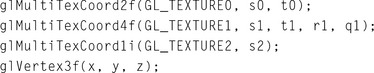
The behavior of the glTexCoord family of routines is specified to update just texture unit zero.
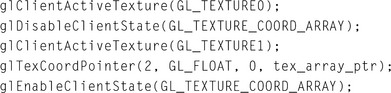
Multitexture also supports vertex arrays for multiple texture coordinate sets. In this case, an active texture paradigm is used. Because vertex arrays are considered client state, the glClientActiveTexture command is added to control which vertex array texture coordinate set the glTexCoordPointer, glEnableClientState, glDisableClientState, and glGetPointerv commands effect or query. To illustrate, this example code fragment provides no texture coordinates for texture unit zero, but provides an array pointing to the data in tex_array_ptr for texture unit one:
Multitexturing also extends the current raster position to contain a distinct texture coordinate set for each supported texture unit. Multitexture support was not provided uniformly throughout OpenGL; evaluator and feedback functionality are not extended to support multiple texture coordinate sets. Evaluators and feedback utilize only texture coordinate set zero.
The glPushAttrib, glPopAttrib, glPushClientAttrib, and glPopClientAttrib push and pop respectively all the respective server or client texture state of all texture units when texture-related state is pushed or popped.
5.9.2 Multitexture Texture Environments
Much of the multitexture functionality, such as texture coordinate generation, texel lookup, and texture filtering, can be thought of as operating independently in each texture unit. But they must interact during the texture environment stage to provide a single fragment color. The multitexture pipeline uses a cascade model to combine the incoming fragment color with the fragment’s texture contribution from each texture unit. The first enabled texture unit uses its state to control how to combine the incoming fragment color with its corresponding texture color.
The resulting color is passed to the next enabled texture unit, where the process is repeated. The texture unit uses its environment state to control how the incoming color (which came from the previous active texture unit), is combined with the corresponding texture color, then passes the resulting color to the next active unit.
This process continues until all the enabled texture units have modified the fragment color. The texture units are accessed by increasing numerical order; texture unit 0 (if active), then texture unit 1 (if active), and so on. Figure 5.11 illustrates the multitexture dataflow.
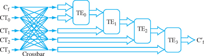
Figure 5.11 Multitexture texture environments. Four texture units are shown; however, the number of units available depends on the implementation. The input fragment color is successively combined with each texture according to the state of the corresponding texture environment, and the resulting fragment color passed as input to the next texture unit in the pipeline.
Multitexture with basic texture environment functionality is extremely useful for streamlining multitexture algorithms such as light maps or environment mapping. But modern multitexture hardware has evolved to support a substantially more flexible facility for combining multiple textures. This evolution is reflected in a number of additions to the texture environment functionality. Multitexturing techniques reach their fullest potential when used with this more advanced version of texture environment. It is implemented in OpenGL through the ARB_texture_env_combine, ARB_texture_env_dot3, and ARB_texture_env_crossbar extensions. The first two extensions was added to core OpenGL 1.3, while the last is in OpenGL 1.4. The following section describes this functionality in more detail.
5.10 Texture Environment
The texturing stage that computes the final fragment color value is called the texture environment function (glTexEnv). This stage takes the filtered texel color (the texture color) and the untextured color that comes from rasterizing the untextured polygon, called the fragment color. In addition to these two input values, the application can also supply an additional color value, called the environment color. The application chooses a method to combine these colors to produce a final color. OpenGL provides a fixed set of methods for the application to choose from.
Each of the methods provided by OpenGL produce a particular effect. One of the most commonly used is the GL_MODULATE environment function. The modulate function multiplies or modulates the polygon’s fragment color with the texel color. Typically, applications generate polygons with per-vertex lighting enabled and then modulate the texture image with the fragment’s interpolated lighted color value to produce a lighted, textured surface.
The GL_REPLACE texture environment10 function is much simpler. It just replaces the fragment color with the texture color. The replace function can be emulated in OpenGL 1.0 by using the modulate environment with a constant white polygon color, though the replace function has a lower computational cost.
The GL_DECAL environment function alpha-blends between the fragment color and an RGBA texture’s texture color, using the texture’s alpha component to control the interpolation; for RGB textures it simply replaces the fragment color. Decal mode is undefined for other texture formats (luminance, alpha, intensity). The GL_BLEND environment function is a little different. It uses the texture value to control the mixing of the fragment color and the application-supplied texture environment color.
5.10.1 Advanced Texture Environment Functionality
Modern graphics hardware has undergone a substantial increase in power and flexibility, adding multiple texture units and new ways to combine the results of the lookup operations. OpenGL has evolved to better use this functionality by adding multitexturing functionality and by providing more flexible and powerful fixed-function texture environment processing. This evolution has culminated in transition from a fixed-function model to a programmable model, adding an interface for programming texturing hardware directly with a special shading language.
As of OpenGL 1.3, three more environment function extensions were added to the core specification. The ARB_texture_env_add extension adds the GL_ADD texture environment function in which the final color is produced by adding the fragment and texture color. This functionality is useful to support additive detail, such as specular highlights, and additive lightmaps.
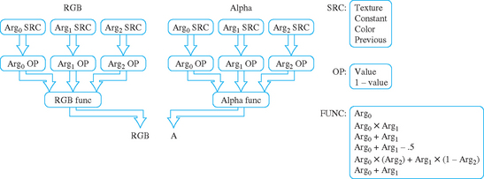
The ARB_texture_env_combine extension provides a fine-grain orthogonal set of fixed-function texture environment settings. This reorganization of texture environment functionality can take better advantage of programmable texturing hardware. When GL_COMBINE is specified, two different texture environment functions can be specified; one for the RGB components and one for the alpha components of the incoming colors. Each environment function is chosen from a corresponding set of RGB and alpha functions.
Unlike previous texture environment functions, the combine functions are generic; they operate on three arguments, named Arg0, Arg1, and Arg2. These arguments are specified with source and operand enumerants for each argument. Like the environment functions themselves, there are distinct sets of source and operand enumerants for RGB and alpha color components. An argument source can be configured to be the filtered texture color GL_TEXTURE, the application-specified texture environment color GL_CONSTANT, the untextured fragment color from the primitive GL_PRIMARY_COLOR, or the color from the previous texture stage GL_PREVIOUS. The components of the argument’s specified color are modified by the operand argument. An operand can choose the RGB or alpha components of the source color, use them unchanged, or invert them (apply a 1 − color operation to each component). Figure 5.12 illustrates the relationships between the components that make up the combine function.
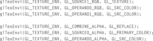
Configuring this new functionality may become clearer with an example. It uses the GL_COMBINE functionality to mimic the GL_MODULATE function. The following command sequence will produce the same effect as GL_MODULATE on an RGB texture:
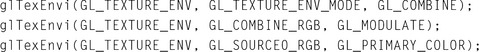
The ARB_texture_env_dot3 extension augments the combine functionality, providing RGB and RGBA dot product RGB functions. Per-pixel dot product functions are useful for a number of techniques, such as implementing a common bump mapping technique.
With OpenGL 1.4 another extension was added to the core; ARB_texture_env_crossbar. This extension also augments the combine interface. Instead of restricting the source of a previously textured color value to the previous texture unit, the crossbar functionality makes it possible to use the output from any previous active texture unit in the texturing chain. This makes texture environment sequences more flexible; for example, a particular texture unit’s output can be used as input by multiple texturing units. This functionality allows the fixed function combine interface to more closely approximate a fully programmable one.
5.10.2 Fragment Programs
The evolution of texture environment functionality has progressed to the point where OpenGL can support fully programmable texture (shading) hardware. The ARB_fragment_program extension defines a programming language that can be loaded in the pipeline through a set of new commands. Programs can be loaded, made current, and have parameter values assigned.
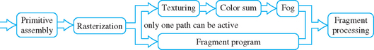
The programming language not only provides a fully programmable replacement for texture environment operations (including support for depth textures), but also supplants the color summation stage (for separate specular color) and fog computations, as shown in Figure 5.13.
Besides a programming language, the fragment program extension provides additional commands for loading, selecting, and modifying fragment programs (which are called program objects). The functionality provided is very similar to that used for texture objects. The glProgramStringARB command loads a new fragment program; it can be made current with glBindProgramARB; and deleted with glDeleteProgramsARB. There are also queries and tests that can be used to retrieve a loaded program, or to check for its existence.
Fragment programs can use environment and local variables, called parameters. A local parameter can be thought of as a static variable, global to the program. Environment parameters are variable values global to all programs in the implementation. All parameters are an array of four floating-point values (eliminating a multitude of dynamic range and precision problems in the fixed-function pipeline). These values can be changed in a loaded program using various forms of glProgramEnvParameter and glProgramLocalParameter. Since these parameters can be modified in a program even after it is loaded, it makes it possible to use a parameterized program multiple ways, without having to reload it.
Going into the details of the fragment programming language is beyond the scope of this book, but some general comments can give some idea of its capabilities. The currently active fragment program operates on fragments generated during rasterization. Fragment programs appear like assembly language, having simple instructions and operands. The instructions have a digital signal processor (DSP) flavor, supporting trigonometric operations such as sine and cosine, dot and cross products, exponentiation, and multiply-add. Special instructions provide texture lookup capability. Instructions operate on vector and scalar floating-point values, they can come from attributes of the rasterized fragment, temporary variables in the program, or parameters that can be modified by the application. There is built-in support for swizzling vector arguments as well as negation.
As mentioned previously, the base extension provides no flow control or looping constructs, but there are conditional set instructions, and instructions that can be used to “kill” (discard) individual fragments. These instructions, in concert with local and environment parameters that can be changed after a program is loaded, make it possible to control (i.e., parameterize) the behavior of a fragment program. The final result of the program execution is a color and depth value that is passed down to the remainder of the fragment pipeline (scissor test, alpha test, etc.).
When available, this extension can replace a significant number of multipass operations with programmable micropass ones. See Section 9.5 for details on the difference between multipass and micropass approaches to complex rendering.
Fragment program functionality is still evolving. There are extensions to this functionality, such as providing conditionals and looping constructs in the language, as well as a set of higher level languages that are “compiled” into fragment programs, such as Cg (NVIDIA, 2004) and GLSL (Kessenich, 2003). Other possible extensions might increase fragment program scope to control more of the fragment processing pipeline, for example, manipulating stencil values. At this time neither fragment or vertex program functionality is part of core OpenGL, but both are expected to be part of OpenGL 2.0. For this reason, and because there are other texts covering fragment and vertex programming, we limit our discussion of them in this book. For detailed information on this extension, look at the documentation on the ARB_fragment_program extension and the OpenGL Shading Language at the opengl.org website.
5.11 Summary
Texture mapping is arguably the most important functionality in OpenGL, and is still undergoing significant evolution. Texture mapping functionality, while complex, is well worth the time to study thoroughly. This chapter describes the basic texture mapping machinery, Chapter 14 describes several “building block” techniques, and many of the other chapters make extensive use of texture mapping algorithms as key parts of the overall technique.
1ARB_texture_non_power_of_two.
2Added in OpenGL 1.3.
33D textures were available as an extension and later became part of the core standard in OpenGL 1.2.
4Introduced in OpenGL 1.1.
5Many texts (Foley et al., 1990; Foley et al., 1994; Rogers, 1997) present this reflection vector formula with a sign reversed, but it is the same fundamental formula. The difference is simply one of convention: the OpenGL U vector points from the eye to the surface vertex (an eye-space position), while many texts use a light vector pointing from the surface to the light.
63D textures were added to OpenGL 1.2; prior to 1.2 they are available as an extension.
7This same functionality for controlling texture level of detail is also available through the SGIS_texture_lod extension.
8Texture objects were added in OpenGL 1.1.
9This functionality was also available earlier as the ARB_multitexture extension.
10Introduced by OpenGL 1.1.