Digital Images and Image Manipulation
Geometric rendering is, at best, half of a good graphics library. Modern rendering techniques combine both geometric and image-based rendering. Texture mapping is only the simplest example of this concept; later chapters in this book cover more sophisticated techniques that rely both on geometry rendering and image processing. This chapter reviews the characteristics of a digital image and outlines OpenGL’s image manipulation capabilities. These capabilities are traditionally encompassed by the pipeline’s “pixel path”, and the blend functionality in the “fragment operations” part of the OpenGL pipeline.
Even if an application doesn’t make use of sophisticated image processing, familiarity with the basics of image representation and sampling theory guides the crafting of good quality images and helps when fixing many problems encountered when rendering and texture mapping.
4.1 Image Representation
The output of the rendering process is a digital image stored as a rectangular array of pixels in the color buffer. These pixels may be displayed on a CRT or LCD display device, copied to application memory to be stored or further manipulated, or re-used as a texture map in another rendering task. Each pixel value may be a single scalar component, or a vector containing a separate scalar value for each color component.
Details on how a geometric primitive is converted to pixels are given in Chapter 6; for now assume that each pixel accurately represents the average color value of the geometric primitives that cover it. The process of converting a continuous function into a series of discrete values is called sampling. A geometric primitive, projected into 2D, can be thought of as defining a continuous function of its spatial coordinates x and y.
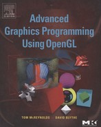
For example, a triangle can be represented by a function fcontinuous(x, y). It returns the color of the triangle when evaluated within the triangle’s extent, then drops to zero if evaluated outside of the triangle. Note that an ideal function has an abrupt change of value at the triangle boundaries. This instantaneous drop-off is what leads to problems when representing geometry as a sampled image. The output of the function isn’t limited to a color; it can be any of the primitive attributes: intensity (color), depth, or texture coordinates; these values may also vary across the primitive. To avoid overcomplicating matters, we can limit the discussion to intensity values without losing any generality.
A straightforward approach to sampling the geometric function is to evaluate the function at the center of each pixel in window coordinates. The result of this process is a pixel image; a rectangular array of intensity samples taken uniformly across the projected geometry, with the sample grid aligned to the x and y axes. The number of samples per unit length in each direction defines the sample rate.
When the pixel values are used to display the image, a reproduction of the original function is reconstructed from the set of sample values. The reconstruction process produces a new continuous function. The reconstruction function may vary in complexity; for example, it may simply repeat the sample value across the sample period
or compute a weighted sum of pixel values that bracket the reconstruction point. Figure 4.1 shows an example of image reconstruction.
When displaying a graphics image, the reconstruction phase is often implicit; the reconstruction is part of the video display circuitry and the physics of the pixel display. For example, in a CRT display, the display circuitry uses each pixel intensity value to adjust the intensity of the electron beam striking a set of phosphors on the screen. This reconstruction function is complex, involving not only properties of the video circuitry, but also the shape, pattern, and physics of the phosphor on the screen. The accuracy of a reconstructed triangle may depend on the alignment of phosphors to pixels, how abruptly the electron beam can change intensity, the linearity of the analog control circuitry, and the design of the digital to analog circuitry. Each type of output device has a different reconstruction process. However, the objective is always the same, to faithfully reproduce the original image from a set of samples.
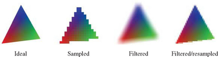
The fidelity of the reproduction is a critical aspect of using digital images. A fundamental concern of sampling is ensuring that there are enough samples to accurately reproduce the desired function. The problem is that a set of discrete sample points cannot capture arbitrarily complicated detail, even if we use the most sophisticated reconstruction function. This is illustrated by considering an intensity function that has the similar values at two sample points P1 and P3, but between these points P2 the intensity varies significantly, as shown in Figure 4.2. The result is that the reconstructed function doesn’t reproduce the original function very well. Using too few sample points is called undersampling; the effects on a rendered image can be severe, so it is useful to understand the issue in more detail.
To understand sampling, it helps to rely on some signal processing theory, in particular, Fourier analysis (Heidrich and Seidel, 1998; Gonzalez and Wintz, 1987). In signal processing, the continuous intensity function is called a signal. This signal is traditionally represented in the spatial domain as a function of spatial coordinates. Fourier analysis states that the signal can be equivalently represented as a weighted sum of sine waves of different frequencies and phase offsets. This is a bit of an oversimplification, but it doesn’t affect the result. The corresponding frequency domain representation of a signal describes the magnitude and phase offset of each sine wave component. The frequency domain representation describes the spectral composition of the signal.
The sine wave decomposition and frequency domain representation are tools that help simplify the characterization of the sampling process. From sine wave decomposition, it becomes clear that the number of samples required to reproduce a sine wave must be twice its frequency, assuming ideal reconstruction. This requirement is called the Nyquist limit. Generalizing from this result, to accurately reconstruct a signal, the sample rate must be at least twice the rate of the maximum frequency in the original signal. Reconstructing an undersampled sine wave results in a different sine wave of a lower frequency. This low-frequency version is called an alias. An aliased signal stands in for the original, since at the lower sampling frequency, the original signal and its aliases are indistinguishable. Aliased signals in digital images give rise to the familiar artifacts of jaggies, or staircasing at object boundaries. Techniques for avoiding aliasing artifacts during rasterization are described in Chapter 10.
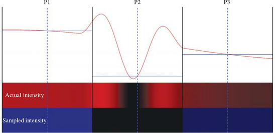
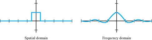
Frequency domain analysis also points to a technique for building a reconstruction function. The desired function can be found by converting its frequency domain representation to one in the spatial domain. In the frequency domain, the ideal function is straightforward; the function that captures the frequency spectrum of the original image is a comb function. Each “tooth” of the comb encloses the frequencies in the original spectrum; in the interests of simplicity, the comb is usually replaced with a single “wide tooth” or box that encloses all of the original frequencies (Figure 4.3). Converting this box function to the spatial domain results in the sinc function. Signal processing theory provides a framework for evaluating the fidelity of sampling and reconstruction in both the spatial and frequency domain. Often it is more useful to look at the frequency domain analysis since it determines how individual spectral components (frequencies) are affected by the reconstruction function.
4.2 Digital Filtering
Consider again the original continuous function representing a primitive. The function drops to zero abruptly at the edge of the polyon, representing a step function at the polygon boundaries. Representing a step function in the frequency domain results in frequency components with non-zero values at infinite frequencies. Avoiding creating undersampling artifacts when reconstructing a sampled step function requires changing the input function, or the way it is sampled. In essence, the boundaries of the polygon must be “smoothed” so that the transition can be represented by a bounded frequency representation. The frequency bound is chosen so that it can be captured by the samples. This process is an application of filtering.
As alluded to in the discussion above, filtering goes hand in hand with the concept of sampling and reconstruction. Conceptually, filtering applies a function to an input signal to produce a new one. The filter modifies some of the properties of the original signal, such as removing frequency components above or below some threshold (low- and high-pass filters). With digital images, filtering is often combined with reconstruction followed by resampling. Reconstruction produces a continuous signal for the filter to operate on and resampling produces a set of sample values from the filtered signal, possibly at a different sample rate. The term filter is frequently used to mean all three parts: reconstruction, filtering, and resampling. The objective of applying the filter is most often to transform the spectral composition of the signal.
As an example, consider the steps to produce a new version of an image that is half the size in the x and y dimensions. One way to generate the new image is to copy every second pixel into the new image. This process can be viewed as a reconstruction and resampling process. By skipping every other pixel (which represents a sample of the original image), we are sampling at half the rate used to capture the original image. Reducing the rate is a form of undersampling, and will introduces new signal aliases.
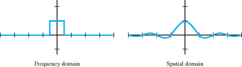
These aliased signals can be avoided by eliminating the frequency components that cannot be represented at the new, lower sampling rate. This is done by applying a low-pass filter during signal reconstruction, before the new samples are computed. There are many useful low-pass filter functions; one of the simplest is the box filter. The 2×2-box filter computes a new sample by taking an equally weighted average of four adjacent samples. The effect of the box filter on the spectrum of the signal can be evaluated by converting it to the frequency domain. Although simple, the box filter isn’t a terrific low-pass filter, it corresponds to multiplying the spectrum by a sinc function in the frequency domain (Figure 4.4). This function doesn’t cut off the high frequencies very cleanly, and leads to its own set of artifacts.
4.3 Convolution
Both the reconstruction and spectrum-shaping filter functions compute weighted sums of surrounding sample values. These weights are values from a second function and the computation of the weighted sum is called convolution. In one dimension, the convolution of two continuous functions f(x) and g(x) produces a third function:
g(x) is referred to as the filter. The integral only needs to be evaluated over the range where g(x−τ) is non-zero, called the support of the filter.
The discrete form of convolution operates on two arrays, the discretized signal F[x] and the convolution kernel G[0 … (width − 1)]. The value of width defines the support of the filter and Equation 4.1 becomes:
The 1D discrete form is extended to two dimensions as:
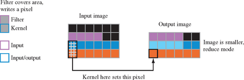
As shown in Figure 4.5, a convolution kernel is positioned over each pixel in an image to be convolved, and an output pixel is generated. The kernel can be thought of as an array of data values; these values are applied to the input pixels that the convolution kernel covers. Multiplying and summing the kernel against its footprint in the image creates a new pixel value, which is used to update the convolved image. Note that the results of a previous convolution step don’t affect any subsequent steps; each output pixel is independent of the surrounding output pixels.
The formalization and use of the convolution operation isn’t accidental; it relates back to Fourier analysis. The significance of convolution in the spatial domain is that it is equivalent to multiplying the frequency domain representations of the two functions. This means that a filter with some desired properties can be constructed in the frequency domain and then converted to the spatial domain to perform the filtering. In some cases it is more efficient to transform the signal to the frequency domain, perform the multiplication, and convert back to the spatial domain. Discussion of techniques for implementing filters and of different types of filters is in Chapter 12. For the rest of this chapter we shall describe the basic mechanisms OpenGL provides for operating on images.
4.4 Images in OpenGL
The OpenGL API contains a pixel pipeline for performing many traditional image processing operations, such as scaling or rotating an image. The use of hybrid 3D rasterization and image processing techniques has increased over recent years, giving rise to the term image-based rendering [MB95, LH96, GGSC96]. More recent versions of OpenGL have increased the power and sophistication of the pixel pipeline to match the demand for these capabilities.
Image processing operations can be applied while loading pixel images and textures into OpenGL, reading them back to the host, or copying them. The ability to modify textures during loading operations and to modify framebuffer contents during copy operations provides high-performance paths for image processing operations. These operations may be performed entirely within the graphics accelerator, so they can be independent of the performance of the host.
OpenGL distinguishes between several types of images. Pixel images, or pixmaps are transferred using the glDrawPixels command. Pixmaps can represent index or RGB color values, depth values, or stencil values. Bitmap images are a special case of pixmaps consisting of single-bit per-pixel images. When bitmaps are drawn they are expanded into constant index or RGB colors. The glBitmap command is used to draw bitmaps and includes extra support for adjusting the current drawing position so that text strings can be efficiently rendered and positioned as bitmap glyphs. A third image type is texture images. Texture images are virtually identical to pixmap images, but special commands are used to transfer texture image data to texture objects. Texture maps are specialized to support 1D, 2D and 3D images as well as 6-sided cube maps. Texture maps also include support for image pyramids (also called mipmaps), used to provide additional filtering support.
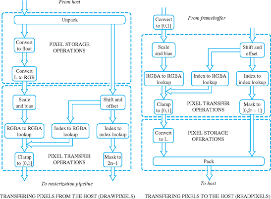
Figure 4.6 shows a block diagram of the base OpenGL pixel pipeline. The pipeline is divided into two major blocks of operations: pixel storage operations that control how pixels are read or written to application memory, and pixel transfer operations that operate on streams of pixels in a uniform format inside the pipeline. At the end of the pixel pipeline is a pixel zoom operation that allow simple (unfiltered) scaling of images. After the zoom operation, pixel images are converted into individual fragments, where the fragments are processed in exactly the same way as fragments generated from geometry.
4.5 Positioning Images
Each of the image types (pixmaps, bitmaps, and textures) has slight variations in how they are specified to the pipeline. Both pixmaps and bitmaps share the notion of the current raster position defining the window coordinates of the bottom left corner of the image. The raster position is specified and transformed as a 3D homogeneous point similar to the vertices of other geometric primitives. The raster position also undergoes frustum clip testing and the entire primitive is discarded if the raster position is outside the frustum. The window coordinate raster position can be manipulated directly using the glWindowPos1 or glBitmap commands. Neither the absolute position of the window position command or the result of adding the relative adjustment from the bitmap command are clip tested, so they can be used to position images partially outside the viewport.
The texture image commands have undergone some evolution since OpenGL 1.0 to allow incremental update to individual images. The necessary changes include commands that include offsets within the texture map and the ability to use a null image to initialize texture map with a size but no actual data.
4.6 Pixel Store Operations
OpenGL can read and write images with varying numbers, sizes, packings, and orderings of pixel components into system memory. This diversity in storage formats provides a great deal of control, allowing applications to fine tune storage formats to match external representations and maximize performance or compactness. Inside the pipeline, images are converted to a stream of RGBA pixels at an implementation-specific component resolution. There are few exceptions: depth, stencil, color index, and bitmap images are treated differently since they don’t represent RGBA color values. OpenGL also distinguishes intensity and luminance images from RGBA ones. Intensity images are single component images that are expanded to RGBA images by copying the intensity to each of the R, G, B, and A components.2 Luminance images are also single component images, but are expanded to RGB in the pipeline by copying the luminance to the R component while setting the G and B components to zero.
Pixel storage operations process an image as it is read or written into host memory, converting to and from OpenGL’s internal representation and the application’s memory format. The storage operations do not affect how the image is stored in the framebuffer; that information is implementation-dependent. Pixel storage operations are divided into two symmetric groups: the pack group, controlling how data is stored to host memory, and the unpack group, controlling how image data is read from host memory.
2D images are stored in application memory as regularly spaced arrays, ordered so they can be transfered one row at a time to form rectangular regions. The first row starts at the lowest memory address and the first pixel corresponds to the bottom left pixel of the image when rendered (assuming no geometric transforms). A 3D image is stored as a series of these rectangles, stacked together to form a block of image data starting with the slice nearest to the image pointer, progressively moving to the furthest.
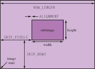
In addition to component ordering and size, the pixel storage modes provide some additional control over the layout of images in memory, including the ability to address a subrectangle within a memory image. Figure 4.7 shows the layout of an image in memory and the effect of the alignment and spacing parameters. Additional parameters facilitate portability between different platforms: byte swapping within individual component representations and bit ordering for bitmaps.
From an application writer’s point of view, the pixel store operations provide an opportunity for the OpenGL pipeline to efficiently accelerate common conversion operations, rather than performing the operations on the host. For example, if a storage format operates with 16-bit (unsigned short) components, OpenGL can read and write those directly. Similarly, if a very large image is to be operated on in pieces, OpenGL’s ability to transfer a subrectangle can be exploited, avoiding the need to extract and transfer individual rows of the subrectangle.
One feature that OpenGL does not provide is support for reading images directly from files. There are several reasons for this: it would be difficult to support all the existing image file formats, and keep up with their changes. Providing a simple file access format for all PC architectures would probably not result in the maximum performance implementation. It is also generally better for an application to control the I/O operations themselves. Having no file format also keeps OpenGL cleanly separated from operating system dependencies such as file I/O.
Even if a file interface was implemented, it wouldn’t be sufficient for some applications. In some cases, it can be advantageous to stream image data directly to the graphics pipeline without first transferring the data into application memory. An example is streaming live video from a video capture device. Some vendors have supported this by creating an additional window-like resource that acts as a proxy for the video stream as part of the OpenGL embedding layer. The video source is bound as a read-only window and pixel copy operations are used to read from the video source and push the stream through the pixel pipeline. More details on the platform embedding layer are covered in Chapter 7.
For these reasons OpenGL has no native texture image format, external display list format, or any entrenched dependency on platform capabilities beyond display resource management.
4.7 Pixel Transfer Operations
Pixel transfer operations provide ways of operating on pixel values as they are moved to, read from, or copied within the framebuffer; or as pixels are moved to texture maps. In the base pipeline there are two types of transfer operations: scale and bias and pixel mapping.
4.7.1 Scale and Bias
Scale operations multiply each pixel component by a constant scale factor. The bias operation follows the scale and adds a constant value. RGBA and depth components are operated on with floating-point scales and biases. Analogous operations for indexed components (color index and stencil) use signed integer shift and offset values. Scale and bias operations allow simple affine remapping of pixel components. One example of scale and bias is changing the range of pixel values from [0, 1] to [0.5, 1] for later computations using biased arithmetic. Pixel operations are performed using signed arithmetic and the pixel storage modes support signed component representations; however, at the end of the transfer pipeline component values are clamped to the [0, 1] range.
4.7.2 Pixel Mapping Operations
Pixel mapping operations apply a set of one-dimensional lookup tables to each pixel, making it possible to remap its color components. There are multiple lookup tables, each handling a specific color component. For RGBA colors, there are four maps for converting each color component independently. For indexed colors, there is only one map. Four maps are available for converting indexed colors to RGBA.
A lookup table group applies an application-defined, non-linear transform to image pixels at a specific point in the pixel pipeline. The contents of the lookup tables describe the function; the size of the tables, also application-specified, sets the resolution of the transform operation. Some useful lookup table transforms are: gamma correction, image thresholding, and color inversion. Unfortunately, this feature has an important limitation: a lookup applied to one component cannot change the value of any other component in the pixel.
4.8 ARB Imaging Subset
The OpenGL ARB has defined an additional set of features to significantly enhance OpenGL’s basic image processing capabilities. To preserve OpenGL’s role as an API that can run well on a wide range of graphics hardware, these resource-intensive imaging features are not part of core OpenGL, but grouped into an imaging extension, with the label GL_ARB_imaging.
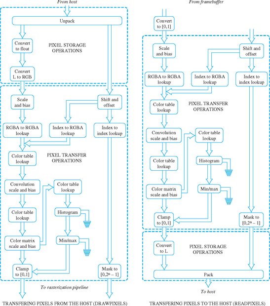
The imaging subset adds convolution, color matrix transform, histogram, and minmax statistics to the pixel transfer block, connecting them with additional color lookup tables. It also adds some additional color buffer blending functionality. Figure 4.8 shows a block diagram of the extended pixel processing pipeline.
4.8.1 Convolution
The imaging subset defines 1D and 2D convolution operations, applied individually to each color component. The maximum kernel width is implementation-dependent but is typically in the range of 7 to 11 pixels. Convolution support includes additional modes for separable 2D filters allowing the filter to be processed as two 1D filters. It also provides different border modes allowing the application different ways of handling the image boundary. Convolution operations, including methods for implementing them without using the imaging subset, are described in more detail in Chapter 12.
A convolution filter is treated similarly to an OpenGL pixel image, except for implementation-specific limitations on the maximum filter dimensions. A filter is loaded by transferring an image to a special OpenGL target. Only pixel storage operations are available to process a filter image while it is being loaded.
4.8.2 Color Matrix Transform
OpenGL’s color matrix provides a 4×4 matrix transform that operates on pixel color components. Each color component can be modified as a linear function of the other components in the pixel. This can’t be done with color lookup tables, since they operate independently on each color component. The matrix is manipulated using the same commands available for manipulating the modelview, texture, and projection matrices.
4.8.3 Histogram
The histogram operation divides each RGBA pixel in the image into four separate color components. Each color component is categorized by its intensity and a counter in the corresponding bin for that component is incremented. The results are kept in four arrays, one for each color component. Effectively, the arrays record the number of occurrences of each intensity range. The size of each range or bin is determined by the length of the application-specified array. For example, a 2-element array stores separate counts for intensity ranges 0 ≤ i < 0.5 and 0.5 <i ≤ 1. The maximum size of the array is implementation-dependent and can be determined using the proxy mechanism.
Histogram operations are useful for analyzing an image by measuring the distribution of its component intensity values. The results can also be used as parameters for other pixel operations. The image may be discarded after the histogram operation is performed, if the image itself is not of interest.
4.8.4 MinMax
The minmax operation looks through all the pixels in an image, finding the largest and smallest intensity value for each color component. The results are saved in a set of two-element arrays, each array corresponding to a different color component. The application can also specify that the image be discarded after minmax information is generated.
4.8.5 Color Tables
Color tables provide additional lookup tables in the OpenGL pixel transfer pipeline. Although the capabilities of color tables and pixel maps are similar, color tables reflect an evolutionary improvement over pixel maps, making them easier to use. Color tables only operate on color components, including luminance and intensity (not color indices, stencil, or depth). Color tables can be defined that affect only a subset of the color components, leaving the rest unmodified.
Color tables are specified as images (like convolution filters). Specifying the complete table at once enables better performance when updating tables often, compared to specifying pixel maps one component at a time. The capability to leave selected components unchanged parallels a similar capability in texturing; this design is simpler than the corresponding functionality in pixel maps, which requires loading an identity map to leave a component unmodified. Color tables don’t operate on depth, stencil, or color index values since those operations don’t occur frequently in applications; the existing pixel map functionality is adequate for these cases.
The additional tables are defined at places in the pipeline where a component normalization operation is likely to be required: before convolution (GL_COLOR_TABLE), after convolution (GL_POST_CONVOLUTION_COLOR_TABLE), and after the color matrix operations (GL_POST_COLOR_MATRIX_COLOR_TABLE). Sometimes normalization operation can be implemented more efficiently using scale and bias operations. To support this, the latter two color tables are preceded by scale and bias operators which may be used in conjunction with, or instead of, the corresponding color tables.
4.8.6 Blend Equation and Constant Color Blending
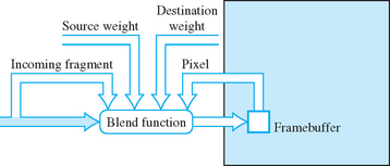
Beyond the pixel path, OpenGL provides an opportunity for the application to manipulate the image in the fragment operations path. OpenGL’s blending function supports additive operations, where scaled versions of the source and destination pixel are added together:
In the equation above, S and D are the source and destination scale factors. Figure 4.9 shows the relationships between the source fragment, target pixel, and source and destination weighting factors. If the glBlendEquation command is supported,3 OpenGL defines additional equations for generating the final pixel value from the source and destination pixels. The new equations are:

The ARB imaging extension includes an additional blending feature, constant color blending, providing more ways to manipulate the image being blended. Constant color blending adds an additional constant blending factor specified by the application. It is usable as either a source or destination blending factor. This functionality makes it possible for the application to introduce an additional color, set by glBlendColor, that can be used to scale the source or destination image during blending.
Both the blend equation and constant color blending functionality were promoted to the base standard in OpenGL 1.4, since they are useful in many other algorithms besides those for image processing. As with texture mapping (see Section 5.14), OpenGL provides proxy support on convolution filters and lookup tables in the pixel pipeline. These are needed to help applications work within the limits an implementation may impose for these images.
4.9 Off-Screen Processing
Image processing or rendering operations don’t always have to produce a transient image for display as part of an application. Some applications may generate images and save them to secondary storage for later use. Batches of images may be efficiently processed without need for operator intervention, for example, filtering an image sequence captured from some other source. Also, some image processing operations may use multiple images to generate the final one. For situations such as these, off-screen storage is useful for holding intermediate images or for accumulating the final result. Support for off-screen rendering is part of the platform embedding layer and is described in Section 7.4.
4.10 Summary
The OpenGL image pipeline is still undergoing evolution. With the transition to a more programmable pipeline, some image manipulation operations can be readily expressed in fragment processing, but many sophisticated operations still require specialized support or more complex algorithms that will be described in Chapter 12.
Image representation and manipulation are essential to the rendering pipeline, not only for generating the final image for viewing, but as part of the rendering process itself. In the next chapter, we will describe the role of images in the texture mapping process. All of the representation issues and the pipeline mechanisms for manipulating images play an important part in the correct application of texture mapping.