Image Processing Techniques
A comprehensive treatment of image processing techniques is beyond the scope of this book. However, since image processing is such a powerful tool, even a subset of image processing techniques can be useful, and is a powerful adjunct to computer graphics approaches. Some of the more fundamental processing algorithms are described here, along with methods for accelerating them using the OpenGL pipeline.
12.1 OpenGL Imaging Support
Image processing is an important component of applications used in the publishing, satellite imagery analysis, medical, and seismic imaging fields. Given its importance, image processing functionality has been added to OpenGL in a number of ways. A bundle of extensions targeted toward accelerating common image processing operations, referred to as the ARB imaging subset, is defined as part of the OpenGL 1.2 and later specifications. This set of extensions includes the color matrix transform, additional color lookup tables, 2D convolution operations, histogram, min/max color value tracking, and additional color buffer blending functionality. These extensions are described in Section 4.8. While these extensions are not essential for all of the image processing techniques described in this chapter, they can provide important performance advantages.
Since the imaging subset is optional, not all implementations of OpenGL support them. If it is advertised as part of the implementation, the entire subset must be implemented. Some implementations provide only part of this functionality by implementing a subset of the imaging extensions, using the EXT versions. Important functionality, such as the color lookup table (EXT_color_table) and convolution (EXT_convolution) can be provided this way.
With the evolution of the fragment processing pipeline to support programmability, many of the functions provided by the imaging subset can be implemented using fragment programs. For example, color matrix arithmetic becomes simple vector operations on color components, color lookup tables become dependent texture reads with multitexture, convolution becomes multiple explicit texture lookup operations with a weighted sum. Other useful extensions, such as pixel textures, are implemented using simple fragment program instructions. However, other image subset operations such as histogram and minmax don’t have direct fragment program equivalents; perhaps over time sufficient constructs will evolve to efficiently support these operations.
Even without this extended functionality, the basic imaging support in OpenGL, described in Chapter 4, provides a firm foundation for creating image processing techniques.
12.2 Image Storage
The multipass concept described in Chapter 9 also applies to image processing. To combine image processing elements into powerful algorithms, the image processing operations must be coupled with some notion of temporary storage, or image variables, for intermediate results. There are three main locations for storing images: in application memory on the host, in a color buffer (back, front, aux buffers, and stereo buffers), or in a texture. A fourth storage location, off-screen memory in pbuffers, is available if the implementation supports them. Each of these storage areas can participate in image operations in one form or another. The biggest difference occurs between images stored as textures and those stored in the other buffers types. Texture images are manipulated by drawing polygonal geometry and operating on the fragment values during rasterization and fragment processing.
Images stored in host memory, color buffers, or pbuffers can be processed by the pixel pipeline, as well as the rasterization and fragment processing pipeline. Images can be easily transferred between the storage locations using glDrawPixels and glReadPixels to transfer images between application memory and color buffers, glCopyTexImage2D to copy images from color buffers to texture memory, and by drawing scaled textured quadrilaterals to copy texture images to a color buffer. To a large extent the techniques discussed in this chapter can be applied regardless of where the image is stored, but some techniques may be more efficient if the image is stored in one particular storage area over another.
If an image is to be used repeatedly as a source operand in an algorithm or by applying the algorithm repeatedly using the same source, it’s useful to optimize the location of the image for the most efficient processing. This will invariably require moving the image from host memory to either texture memory or a color buffer.
12.3 Point Operations
Image processing operations are often divided into two broad classes: point-based and region-based operations. Point operations generate each output pixel as a function of a single corresponding input pixel. Point operations include functions such as thresholding and color-space conversion. Region-based operations calculate a new pixel value using the values in a (usually small) local neighborhood. Examples of region-based operations include convolution and morphology operations.
In a point operation, each component in the output pixel may be a simple function of the corresponding component in the input pixel, or a more general function using additional, non-pixel input parameters. The multipass toolbox methodology outlined in Section 9.3, i.e., building powerful algorithms from a “programming language” of OpenGL operations and storage, is applied here to implement the algorithms outlined here.
12.3.1 Color Adjustment
A simple but important local operation is adjusting a pixel’s color. Although simple to do in OpenGL, this operation is surprisingly useful. It can be used for a number of purposes, from modifying the brightness, hue or saturation of the image, to transforming an image from one color space to another.
12.3.2 Interpolation and Extrapolation
Haeberli and Voorhies (1994) have described several interesting image processing techniques using linear interpolation and extrapolation between two images. Each technique can be described in terms of the formula:
The equation is evaluated on a per-pixel basis. I0 and I1 are the input images, O is the output image, and x is the blending factor. If x is between 0 and 1, the equations describe a linear interpolation. If x is allowed to range outside [0, 1], the result is extrapolation.
In the limited case where 0 ≤ x ≤ 1, these equations may be implemented using constant color blending or the accumulation buffer. The accumulation buffer version uses the following steps:
1. Draw I0 into the color buffer.
2. Load I0, scaling by (1 − x): glAccum(GL_LOAD, (1-x)).
3. Draw I1 into the color buffer.
It is assumed that component values in I0 and I1 are between 0 and 1. Since the accumulation buffer can only store values in the range [−1, 1], for the case x < 0 or x > 1, the equation must be implemented in a such a way that the accumulation operations stay within the [−1, 1] constraint. Given a value x, equation Equation 12.1 is modified to prescale with a factor such that the accumulation buffer does not overflow. To define a scale factor s such that:
Equation 12.1 becomes:
and the list of steps becomes:
2. Draw I0 into the color buffer.
3. Load I0, scaling by ![]() : glAccum(GL_LOAD, (1-x)/s).
: glAccum(GL_LOAD, (1-x)/s).
4. Draw I1 into the color buffer.
The techniques suggested by Haeberli and Voorhies use a degenerate image as I0 and an appropriate value of x to move toward or away from that image. To increase brightness, I0 is set to a black image and x > 1. Saturation may be varied using a luminance version of I1 as I0. (For information on converting RGB images to luminance, see Section 12.3.5.) To change contrast, I0 is set to a gray image of the average luminance value of I1. Decreasing x (toward the gray image) decreases contrast; increasing x increases contrast. Sharpening (unsharp masking) may be accomplished by setting I0 to a blurred version of I1. These latter two examples require the application of a region-based operation to compute I0, but once I0 is computed, only point operations are required.
12.3.3 Scale and Bias
Scale and bias operations apply the affine transformation Cout = sCin + b to each pixel. A frequent use for scale and bias is to compress the range of the pixel values to compensate for limited computation range in another part of the pipeline or to undo this effect by expanding the range. For example, color components ranging from [0, 1] are scaled to half this range by scaling by 0.5; color values are adjusted to an alternate signed representation by scaling by 0.5 and biasing by 0.5. Scale and bias operations may also be used to trivially null or saturate a color component by setting the scale to 0 and the bias to 0 or 1.
Scale and bias can be achieved in a multitude of ways, from using explicit pixel transfer scale and bias operations, to color matrix, fragment programs, blend operations or the accumulation buffer. Scale and bias operations are frequently chained together in image operations, so having multiple points in the pipeline where they can be performed can improve efficiency significantly.
12.3.4 Thresholding
Thresholding operations select pixels whose component values lie within a specified range. The operation may change the values of either the selected or the unselected pixels. A pixel pattern can be highlighted, for example, by setting all the pixels in the pattern to 0. Pixel maps and lookup tables provide a simple mechanism for thresholding using individual component values. However, pixel maps and lookup tables only allow replacement of one component individually, so lookup table thresholding is trivial only for single component images.
To manipulate all of the components in an RGB pixel, a more general lookup table operation is needed, such as pixel textures, or better still, fragment programs. The operation can also be converted to a multipass sequence in which individual component selection operations are performed, then the results combined together to produce the thresholded image. For example, to determine the region of pixels where the R, G, and B components are all within the range [25, 75], the task can be divided into four separate passes. The results of each component threshold operation are directed to the alpha channel; blending is then used to perform simple logic operations to combine the results:
1. Load the GL_PIXEL_MAP_A_TO_A with a values that map components in the range [0.25, 0.75] to 1 and everything else to 0. Load the other color pixel maps with a single entry that maps all components to 1 and enable the color pixel map.
2. Clear the color buffer to (1, 1, 1, 0) and enable blending with source and destination blend factors GL_SRC_ALPHA, GL_SRC_ALPHA.
3. Use glDrawPixels to draw the image with the R channel in the A position.
4. Repeat the previous step for the G and B channels.
5. At this point the color buffer has 1 for every pixel meeting the condition 0.25 ≤ x ≤ 0.75 for the three color components. The image is drawn one more time with the blend function set to glBlendFunc(GL_DST_COLOR, GL_ZERO) to modulate the image.
One way to draw the image with the R, G, or B channels in the A position is to use a color matrix swizzle as described in Section 9.3.1. Another approach is to pad the beginning of an RGBA image with several extra component instances, then adjust the input image pointer to glDrawPixels by a negative offset. This will ensure that the desired component starts in the A position. Note that this approach works only for 4-component images in which all of the components are equal size.
12.3.5 Conversion to Luminance
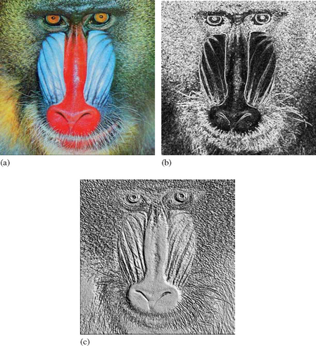
A color image is converted to a luminance image (Figure 12.1) by scaling each component by its weight in the luminance equation.

The recommended weight values for Rw, Gw, and Bw are 0.2126, 0.7152, and 0.0722, respectively, from the ITU-R BT.709-5 standard for HDTV. These values are identical to the luminance component from the CIE XYZ conversions described in Section 12.3.8. Some authors have used the values from the NTSC YIQ color conversion equation (0.299, 0.587, and 0.114), but these values are inapproriate for a linear RGB color space (Haeberli, 1993). This operation is most easily achieved using the color matrix, since the computation involves a weighted sum across the R, G, and B color components.
In the absence of color matrix or programmable pipeline support, the equivalent result can be achieved, albeit less efficiently, by splitting the operation into three passes. With each pass, a single component is transferred from the host. The appropriate scale factor is set, using the scale parameter in a scale and bias element. The results are summed together in the color buffer using the source and destination blend factors GL_ONE, GL_ONE.
12.3.6 Manipulating Saturation
The saturation of a color is the distance of that color from a gray of equal intensity (Foley et al., 1990). Haeberli modifies saturation using the equation:
with Rw, Gw, and Bw as described in the previous section. Since the saturation of a color is the difference between the color and a gray value of equal intensity, it is comforting to note that setting s to 0 gives the luminance equation. Setting s to 1 leaves the saturation unchanged; setting it to − 1 takes the complement of the colors (Haeberli, 1993).
12.3.7 Rotating Hue
Changing the hue of a color can be accomplished by a color rotation about the gray vector (1, 1, 1)t in the color matrix. This operation can be performed in one step using the glRotate command. The matrix may also be constructed by rotating the gray vector into the z-axis, then rotating around that. Although more complicated, this approach is the basis of a more accurate hue rotation, and is shown later. The multistage rotation is shown here (Haeberli, 1993):
1. Load the identity matrix: glLoadIdentity.
2. Rotate such that the gray vector maps onto the z-axis using the glRotate command.
3. Rotate about the z-axis to adjust the hue: glRotate(<degrees>, 0, 0, 1).
Unfortunately, this naive application of glRotate will not preserve the luminance of an image. To avoid this problem, the color rotation about z can be augmented. The color space can be transformed so that areas of constant luminance map to planes perpendicular to the z-axis. Then a hue rotation about that axis will preserve luminance. Since the luminance of a vector (R, G, B) is equal to:
the plane of constant luminance k is defined by:
Therefore, the vector (Rw, Gw, Bw) is perpendicular to planes of constant luminance. The algorithm for matrix construction becomes the following (Haeberli, 1993):
2. Apply a rotation matrix M such that the gray vector (1, 1, 1)t maps onto the positive z-axis.
3. Compute (R′w, G′w, B′w)t = M(Rw, Gw, Bw)t. Apply a skew transform which maps (R′w, G′w, B′w)t to (0, 0, B′w)t. This matrix is:
4. Rotate about the z-axis to adjust the hue.
It is possible to create a single matrix which is defined as a function of Rw, Gw, Bw, and the amount of hue rotation required.
12.3.8 Color Space Conversion
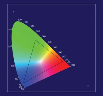
CIE XYZ Conversion The CIE (Commission Internationale de L′Éclairage) color space is the internationally agreed on representation of color. It consists of three spectral weighting curves ![]() called color matching functions for the CIE Standard Observer. A tristimulus color is represented as an XYZ triple, where Y corresponds to luminance and X and Z to the response values from the two remaining color matching functions. The CIE also defines a representation for “pure” color, termed chromaticity consisting of the two values
called color matching functions for the CIE Standard Observer. A tristimulus color is represented as an XYZ triple, where Y corresponds to luminance and X and Z to the response values from the two remaining color matching functions. The CIE also defines a representation for “pure” color, termed chromaticity consisting of the two values
A chromaticity diagram plots the chromaticities of wavelengths from 400 nm to 700 nm resulting in the inverted “U” shape shown in Figure 12.2. The shape defines the gamut of visible colors. The CIE color space can also be plotted as a 3D volume, but the 2D chromaticity projection provides some useful information. RGB color spaces project to a triangle on the chromaticity diagram, and the triangle defines the gamut of the RGB color space. Each of the R, G, and B primaries form a vertex of the triangle. Different RGB color spaces map to different triangles in the chromaticity diagram. There are many standardized RGB color space definitions, each with a different purpose. Perhaps the most important is the ITU-R BT.709-5 definition. This RGB color space defines the RGB gamut for digital video signals and roughly matches the range of color that can be reproduced on CRT-like display devices. Other RGB color spaces represent gamuts of different sizes. For example, the Adobe RGB (1998) color space projects to a larger triangle and can represent a large range of colors. This can be useful for transfer to output devices that are capable of reproducing a larger gamut. Note that with a finite width color representation, such as 8-bit RGB color components, there is a trade-off between the representable range of colors and the ability to differentiate between distinct colors. That is, there is a trade-off between dynamic range and precision.
To transform from BT.709 RGB to the CIE XYZ color space, use the following matrix:
The XYZ values of each of the R, G, and B primaries are the columns of the matrix. The inverse matrix is used to map XYZ to RGBA (Foley et al., 1990). Note that the CIE XYZ space can represent colors outside the RGB gamut. Care should be taken to ensure the XYZ colors are “clipped” as necessary to produce representable RGB colors (all components lie within the 0 to 1 range).
Conversion between different RGB spaces is achieved by using the CIE XYZ space as a common intermediate space. An RGB space definition should include CIE XYZ values for the RGB primaries. Color management systems use this as one of the principles for converting images from one color space to another.
CMY Conversion The CMY color space describes colors in terms of the subtractive primaries: cyan, magenta, and yellow. CMY is used for hardcopy devices such as color printers, so it is useful to be able to convert to CMY from RGB color space. The conversion from RGB to CMY follows the equation (Foley, et al., 1990):
CMY conversion may be performed using the color matrix or as a scale and bias operation. The conversion is equivalent to a scale by − 1 and a bias by +1. Using the 4 × 4 color matrix, the equation can be restated as:
To produce the correct bias from the matrix multiply, the alpha component of the incoming color must be equal to 1. If the source image is RGB, the 1 will be added automatically during the format conversion stage of the pipeline.
A related color space, CMYK, uses a fourth channel (K) to represent black. Since conversion to CMYK requires a min() operation, it cannot be done using the color matrix.
The OpenGL extension EXT_CMYKA adds support for CMYK and CMYKA (CMYK with alpha). It provides methods to read and write CMYK and CMYKA values stored in system memory (which also implies conversion to RGB and RGBA, respectively).
YIQ Conversion The YIQ color space was explicitly designed to support color television, while allowing backwards compatibility with black and white TVs. It is still used today in non-HDTV color television broadcasting in the United States. Conversion from RGBA to YIQA can be done using the color matrix:
(Generally, YIQ is not used with an alpha channel so the fourth component is eliminated.) The inverse matrix is used to map YIQ to RGBA (Foley et al., 1990):
HSV Conversion The hue saturation value (HSV) model is based on intuitive color characteristics. Saturation characterizes the purity of the color or how much white is mixed in, with zero white being the purest. Value characterizes the brightness of the color. The space is defined by a hexicone in cylindrical coordinates, with hue ranging from 0 to 360 degrees (often normalized to the [0, 1] range), saturation from 0 to 1 (purest), and value from 0 to 1 (brightest). Unlike the other color space conversions, converting to HSV can’t be expressed as a simple matrix transform. It can be emulated using lookup tables or by directly implementing the formula:
The conversion from HSV to RGB requires a similar strategy to implement the formula:
12.4 Region-based Operations
A region-based operation generates an output pixel value from multiple input pixel values. Frequently the input value’s spatial coordinates are near the coordinates of the output pixel, but in general an output pixel value can be a function of any or all of the pixels in the input image. An example of such a function is the minmax operation, which computes the minimum and maximum component values across an entire pixel image. This class of image processing operations is very powerful, and is the basis of many important operations, such as edge detection, image sharpening, and image analysis.
OpenGL can be used to create several toolbox functions to make it easier to perform non-local operations. For example, once an image is transferred to texture memory, texture mapped drawing operations can be used to shift the texel values to arbitrary window coordinates. This can be done by manipulating the window or texture coordinates of the accompanying geometry. If fragment programs are supported, they can be used to sample from arbitrary locations within a texture and combine the results (albeit with limits on the number of instructions or samples). Histogram and minmax operations can be used to compute statistics across an image; the resulting values can later be used as weighting factors.
12.4.1 Contrast Stretching
Contrast stretching is a simple method for improving the contrast of an image by linearly scaling (stretching) the intensity of each pixel by a fixed amount. Images in which the intensity values are confined to a narrow range work well with this algorithm. The linear scaling equation is:
where min(Iin) and max(Iin) are the minimum and maximum intensity values in the input image. If the intensity extrema are already known, the stretching operation is really a point operation using a simple scale and bias. However, the search operation required to find the extrema is a non-local operation. If the imaging subset is available, the minmax operation can be used to find them.
12.4.2 Histogram Equalization
Histogram equalization is a more sophisticated technique, modifying the dynamic range of an image by altering the pixel values, guided by the intensity histogram of that image. Recall that the intensity histogram of an image is a table of counts, each representing a range of intensity values. The counts record the number of times each intensity value range occurs in the image. For an RGB image, there is a separate table entry for each of the R, G, and B components. Histogram equalization creates a non-linear mapping, which reassigns the intensity values in the input image such that the resultant images contain a uniform distribution of intensities, resulting in a flat (or nearly flat) histogram. This mapping operation is performed using a lookup table. The resulting image typically brings more image details to light, since it makes better use of the available dynamic range.
12.5 Reduction Operations
The minmax and histogram computations are representative of a class of reduction operations in which an entire image is scanned to produce a small number of values. For minmax, two color values are computed and for luminance histograms, an array of counts is computed corresponding to the luminance bins. Other examples include computing the average pixel value, the sum of all the pixel values, the count of pixel values of a particular color, etc. These types of operations are difficult for two reasons. First, the range of intermediate or final values may be large and not easily representable using a finite width color value. For example, an 8-bit color component can only represent 256 values. However, with increasing support for floating-point fragment computations and floating-point colors, this limitation disappears.
The second problem is more architectural. The reduction algorithms can be thought of as taking many inputs and producing a single (or small number of) outputs. The vertex and fragment processing pipelines excel at processing large numbers of inputs (vertices or fragments) and producing a large number of outputs. Parallel processing is heavily exploited in hardware accelerator architectures to achieve significant processing speed increases. Ideally a reduction algorithm should try to exploit this parallel processing capability. One way to accomplish this is by using recursive folding operations to successively reduce the size of the input data. For example, an n×n image is reduced to an n/2×n/2 image of min or max values of neighbor pixels (texels) using texture mapping and a fragment program to compute the minmax of neighboring values. This processing continues by copying the previous result to a texture map and repeating the steps. This reduces the generated image size by 2 along each dimension in each pass until a 1×1 image is left. For an n×n image it takes 1 + [log2 n] passes to compute the final result, or for an n×m image it takes 1 + [log2(max{n,m})] passes (Figure 12.3).
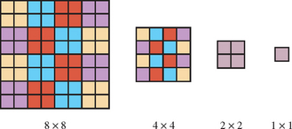
As the intermediate result reduces in size, the degree of available parallelism decreases, but large gains can still be achieved for the early passes, typically until n = 4. When n is sufficiently small, it may be more efficient to transfer the data to the host and complete the computation there if that is the final destination for the result. However, if the result will be used as the input for another OpenGL operation, then it is likely more efficient to complete the computation within the pipeline.
If more samples can be computed in the fragment program, say k×k, then the image size is reduced by k in each dimension at each pass and the number of passes is 1 + [logk(max{n, m})]. The logical extreme occurs when the fragment program is capable of indexing through the entire image in a single fragment program instance, using conditional looping. Conditional looping support is on the horizon for the programmable pipeline, so in the near future the single pass scenario becomes viable. While this may seem attractive, it is important to note that executing the entire algorithm in a single fragment program eliminates all of the inherent per-pixel parallelism. It is likely that maintaining some degree of parallelism throughout the algorithm makes more effective use of the hardware resources and is therefore faster.
Other reduction operations can be computed using a similar folding scheme. For example, the box-filtered mipmap generation algorithm described later in Section 14.15 is the averaging reduction algorithm in disguise. Futhermore, it doesn’t require a fragment program to perform the folding computations. Other reduction operations may also be done using the fixed-function pipeline if they are simple sums or counts.
The histogram operation is another interesting reduction operation. Assuming that a luminance histogram with 256 bins is desired, the computation can be performed by using a fragment program to target one bin at a time. A single texel is sampled at a time, generating 0 or 1 for the texel sample depending on whether it is outside or inside the bin range. Framebuffer blending with GL_ONE, GL_ONE factors is used to sum the results. This requires n × n × 256 passes to process the entire image. To improve upon the parallelism, a 256 × 1 quad can be drawn to sample one texel and compare it against all 256 bins at a time. The window x coordinate is used to determine which bin to compare the texel value against. This reduces the number of passes to n×n. To further reduce the number of passes, the fragment program can be modified to sample some small number of texels at a time, for example 4 to 16. This reduces the number of passes to (n × n)/k.
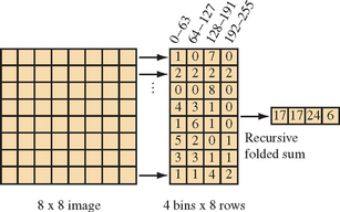
Ideally we would like to achieve the same logarithmic reduction in passes as with the folding scheme. A final improvement to the strategy is to process all rows of the image in parallel, drawing a 256×n quad to index all of the image rows. Multiple rows of output bins are aligned vertically and the y window coordinate chooses the correct row of bins. This leaves a result that is distributed across the multiple rows of bins, so another set of passes is required to reduce the n rows to a single row. This uses the same folding scheme to pairwise sum two rows, one pair of bins, per fragment program. This reduces the number of rows by two in each pass. The end result is an algorithm requiring (1 + [log2 n])n/k passes. Figure 12.4 illustrates the algorithm for a 4-bin histogram on an 8×8 image. Eight rows of bins are simultaneously computed across the columns of the image, producing the final 8 rows of bins. Three sets of folded sums are computed reducing the number of rows of bins by 2 at each step, culminating in the single row of bins on the right.
12.6 Convolution
Convolution is used to perform many common image processing operations. These operations include sharpening, blurring, noise reduction, embossing, and edge enhancement. The mathematics of the convolution operation are described in Section 4.3. This section describes two ways to perform convolutions using OpenGL: with the accumulation buffer and using the convolution operation in the imaging subset.
12.6.1 Separable Filters
Section 4.3 briefly describes the signal processing motivation and the equations behind the general 2D convolution. Each output pixel is the result of the weighted sum of its neighboring pixels. The set of weights is called the filter kernel; the width and height of the kernel determines the number of neighbor pixels (width×height) included in the sum.
In the general case, a 2D convolution operation requires (width×height) multiplications for each output pixel. Separable filters are a special case of general convolution in which the horizontal and vertical filtering components are orthogonal. Mathematically, the filter
can be expressed in terms of two vectors
such that for each (i, j)∈([0..(width − 1)], [0..(height − 1)])
This case is important; if the filter is separable, the convolution operation may be performed using only (width + height) multiplications for each output pixel. Applying the separable filter to Equation 4.3 becomes:
Which simplifies to:
To apply the separable convolution to an image, first apply Grow as though it were a width×1 filter. Then apply Gcol as though it were a 1×height filter.
12.6.2 Convolutions Using the Accumulation Buffer
Instead of using the ARB imaging subset, the convolution operation can be implemented by building the output image in the accumulation buffer. This allows the application to use the important convolution functionality even with OpenGL implementations that don’t support the subset. For each kernel entry G[i][j], translate the input image by (−i,−j) from its original position, then accumulate the translated image using the command glAccum(GL_ACCUM, G[i][j]). This translation can be performed by glCopyPixels but an application may be able to redraw the image shifted using glViewport more efficiently. Width×height translations and accumulations (or width + height if the filter is separable) must be performed.
An example that uses the accumulation buffer to convolve with a Sobel filter, commonly used to do edge detection is shown here. This filter is used to find horizontal edges:
Since the accumulation buffer can only store values in the range [−1, 1], first modify the kernel such that at any point in the computation the values do not exceed this range (assuming the input pixel values are in the range [0, 1]):
3. Translate the input image left by one pixel.
5. Translate the input image left by one pixel.
7. Translate the input image right by two pixels and down by two pixels.
9. Translate the input image left by one pixel.
11. Translate the input image left by one pixel.
13. Return the results to the framebuffer: glAccum(GL_RETURN, 4).
In this example, each pixel in the output image is the combination of pixels in the 3×3 pixel square whose lower left corner is at the output pixel. At each step, the image is shifted so that the pixel that would have been under a given kernel element is under the lower left corner. An accumulation is then performed, using a scale value that matches the kernel element. As an optimization, locations where the kernel value is equal to zero are skipped.
The scale value 4 was chosen to ensure that intermediate results cannot go outside the range [−1, 1]. For a general kernel, an upper estimate of the scale value is computed by summing all of the positive elements of kernel to find the maximum and all of the negative elements to find the minimum. The scale value is the maximum of the absolute value of each sum. This computation assumes that the input image pixels are in the range [0, 1] and the maximum and minimum are simply partial sums from the result of multiplying an image of 1’s with the kernel.
Since the accumulation buffer has limited precision, more accurate results can be obtained by changing the order of the computation, then recomputing scale factor. Ideally, weights with small absolute values should be processed first, progressing to larger weights. Each time the scale factor is changed the GL_MULT operation is used to scale the current partial sum. Additionally, if values in the input image are constrained to a range smaller than [0, 1], the scale factor can be proportionately increased to improve the precision.
For separable kernels, convolution can be implemented using width + height image translations and accumulations. As was done with the general 2D filter, scale factors for the row and column filters are determined, but separately for each filter. The scale values should be calculated such that the accumulation buffer values will never go out of the accumulation buffer range.
12.6.3 Convolution Using Extensions
If the imaging subset is available, convolutions can be computed directly using the convolution operation. Since the pixel transfer pipeline is calculated with extended range and precision, the issues that occur when scaling the kernels and reordering the sums are not applicable. Separable filters are supported as part of the convolution operation as well; they result in a substantial performance improvement.
One noteworthy feature of pipeline convolution is that the filter kernel is stored in the pipeline and it can be updated directly from the framebuffer using glCopyConvolutionFilter2D. This allows an application to compute the convolution filter in the framebuffer and move it directly into the pipeline without going through application memory.
If fragment programs are supported, then the weighted samples can be computed directly in a fragment program by reading multiple point samples from the same texture at different texel offsets. Fragment programs typically have a limit on the number of instructions or samples that can be executed, which will in turn limit the size of a filter that can be supported. Separable filters remain important for reducing the total number of samples that are required. To implement separable filters, separate passes are required for the horizontal and vertical filters and the results are summed using alpha blending or the accumulation buffer. In some cases linear texture filtering can be used to perform piecewise linear approximation of a particular filter, rather than point sampling the function. To implement this, linear filtering is enabled and the sample positions are carefully controlled to force the correct sample weighting. For example, the linear 1D filter computes αT0 + (1−α)T1, where α is determined by the position of the s texture coordinate relative to texels T0 and T1. Placing the s coordinate midway between T0 and T1 equally weights both samples, positioning s 3/4 of the way between T0 and T1 weights the texels by 1/4 and 3/4. The sampling algorithm becomes one of extracting the slopes of the lines connecting adjacent sample points in the filter profile and converting those slopes to texture coordinate offsets.
12.6.4 Useful Convolution Filters
This section briefly describes several useful convolution filters. The filters may be applied to an image using either the convolution extension or the accumulation buffer technique. Unless otherwise noted, the kernels presented are normalized (that is, the kernel weights sum to zero).
Keep in mind that this section is intended only as a very basic reference. Numerous texts on image processing provide more details and other filters, including Myler and Weeks (1993).
Line detection Detection of lines one pixel wide can be accomplished with the following filters:
Gradient Detection (Embossing) Changes in value over 3 pixels can be detected using kernels called gradient masks or Prewitt masks. The filter detects changes in gradient along limited directions, named after the points of the compass (with north equal to the up direction on the screen). The 3×3 kernels are shown here:

Smoothing and Blurring Smoothing and blurring operations are low-pass spatial filters. They reduce or eliminate high-frequency intensity or color changes in an image.
Arithmetic Mean The arithmetic mean simply takes an average of the pixels in the kernel. Each element in the filter is equal to 1 divided by the total number of elements in the filter. Thus, the 3×3 arithmetic mean filter is:
Basic Smooth These filters approximate a Gaussian shape.
High-pass Filters A high-pass filter enhances the high-frequency parts of an image by reducing the low-frequency components. This type of filter can be used to sharpen images.
Laplacian Filter The Laplacian filter enhances discontinuities. It outputs brighter pixel values as it passes over parts of the image that have abrupt changes in intensity, and outputs darker values where the image is not changing rapidly.
Sobel Filter The Sobel filter consists of two kernels which detect horizontal and vertical changes in an image. If both are applied to an image, the results can be used to compute the magnitude and direction of edges in the image. Applying the Sobel kernels results in two images which are stored in the arrays Gh[0..(height−1][0..(width−1)] and Gv[0..(height−1)][0..(width−1)]. The magnitude of the edge passing through the pixel x, y is given by:
(Using the magnitude representation is justified, since the values represent the magnitude of orthogonal vectors.) The direction can also be derived from Gh and Gv:
The 3×3 Sobel kernels are:
12.6.5 Correlation and Feature Detection
Correlation is useful for feature detection; applying correlation to an image that possibly contains a target feature and an image of that feature forms local maxima or pixel value “spikes” in candidate positions. This is useful in detecting letters on a page or the position of armaments on a battlefield. Correlation can also be used to detect motion, such as the velocity of hurricanes in a satellite image or the jittering of an unsteady camera.
The correlation operation is defined mathematically as:
The f*(τ) is the complex conjugate of f(τ), but since this section will limit discussion to correlation for signals which only contain real values, f(τ) can be substituted instead.
For 2D discrete images, Equation 4.3, the convolution equation, may be used to evaluate correlation. In essence, the target feature is stored in the convolution kernel. Wherever the same feature occurs in the image, convolving it against the same image in the kernel will produce a bright spot, or spike.
Convolution functionality from the imaging subset or a fragment program may be used to apply correlation to an image, but only for features no larger than the maximum available convolution kernel size (Figure 12.5). For larger images or for implementation without convolution functionality, convolve with the accumulation buffer technique. It may also be worth the effort to consider an alternative method, such as applying a multiplication in the frequency domain (Gonzalez and Wintz, 1987) to improve performance, if the feature and candidate images are very large.
After applying convolution, the application will need to find the “spikes” to determine where features have been detected. To aid this process, it may be useful to apply thresholding with a color table to convert candidate pixels to one value and non-candidate pixels to another, as described in Section 12.3.4.
Features can be found in an image using the method described below:
1. Draw a small image containing just the feature to be detected.
2. Create a convolution filter containing that image.
3. Transfer the image to the convolution filter using glCopyConvolutionFilter2D.
4. Draw the candidate image into the color buffers.
5. Optionally configure a threshold for candidate pixels:
6. glEnable(GL_CONVOLUTION_2D).
7. Apply pixel transfer to the candidate image using glCopyPixels.
If features in the candidate image are not pixel-exact, for example if they are rotated slightly or blurred, it may be necessary to create a blurry feature image using jittering and blending. Since the correlation spike will be lower when this image matches, it is necessary to lower the acceptance threshold in the color table.
12.7 Geometric Operations
An application may need to magnify an image by a constant factor. OpenGL provides a mechanism to perform simple scaling by replicating or discarding fragments from pixel rectangles with the pixel zoom operation. Zoom factors are specified using glPixelZoom and they may be non-integer, even negative. Negative zoom factors reflect the image about the window coordinate x- and y-axis. Because of its simple operation, an advantage in using pixel zoom is that it is easily accelerated by most implementations. Pixel zoom operations do not perform filtering on the result image, however. In Section 4.1 we described some of the issues with digital image representation and with performing sampling and reconstruction operations on images. Pixel zoom is a form of sampling and reconstruction operation that reconstructs the incoming image by replicating pixels, then samples these values to produce the zoomed image. Using this method to increase or reduce the size of an image introduces aliasing artifacts, therefore it may not provide satisfactory results. One way to minimize the introduction of artifacts is to use the filtering available with texture mapping.
12.7.2 Scaling Using Texture Mapping
Another way to scale an image is to create a texture map from the image and then apply it to a quadrilateral drawn perpendicular to the viewing direction. The interpolated texture coordinates form a regular grid of sample points. With nearest filtering, the resulting image is similar to that produced with pixel zoom. With linear filtering, a weighted average of the four nearest texels (original image pixels) is used to compute each new sample. This triangle filter results in significantly better images when the scale factors are close to unity (0.5 to 2.0) and the performance should be good since texture mapping is typically well optimized. If the scale factor is exactly 1, and the texture coordinates are aligned with texel centers, the filter leaves the image undisturbed. As the scale factors progress further from unity the results become worse and more aliasing artifacts are introduced. Even with its limitations, overall it is a good general technique. An additional benefit: once a texture map has been constructed from the image, texture mapping can be used to implement other geometric operations, such as rotation.
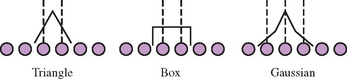
Using the convolution techniques, other filters can be used for scaling operations. Figure 12.6 illustrates 1D examples of triangle, box, and a 3-point Gaussian filter approximation. The triangle filter illustrates the footprint of the OpenGL linear filter. Filters with greater width will yield better results for larger scale factors. For magnification operations, a bicubic (4×4 width) filter provides a good trade-off between quality and performance. As support for the programmable fragment pipeline increases, implementing a bicubic filter as a fragment program will become both straightforward and achieve good performance.
12.7.3 Rotation Using Texture Mapping
There are many algorithms for performing 2D rotations on an image. Conceptually, an algebraic transform is used to map the coordinates of the center of each pixel in the rotated image to its location in the unrotated image. The new pixel value is computed from a weighted sum of samples from the original pixel location. The most efficient algorithms factor the task into multiple shearing transformations (Foley et al., 1990) and filter the result to minimize aliasing artifacts. Image rotation can be performed efficiently in OpenGL by using texture mapping to implement the simple conceptual algorithm. The image is simply texture mapped onto geometry rotated about its center. The texture coordinates follow the rotated vertex coordinates and supply that mapping from rotated pixel position to the original pixel position. Using linear filtering minimizes the introduction of artifacts.
In general, once a texture map is created from an image, any number of geometric transformations can be performed by either modifying the texture or the vertex coordinates. Section 14.11 describes methods for implementing more general image warps using texture mapping.
12.7.4 Distortion Correction
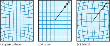
Distortion correction is a commonly used geometric operation. It is used to correct distortions resulting from projections through a lens, or other optically active medium. Two types of distortion commonly occur in camera lenses: pincushion and barrel distortion. Pincushion distortion causes horizontal and vertical lines to bend in toward the center of the image and commonly occurs with zoom or telephoto lenses. Barrel distortion cause vertical and horizontal lines to bend outwards from the center of the image and occurs with wide angle lenses (Figure 12.7).
Distortion is measured as the relative difference of the distance from image center to the distorted position and to the correct position, D = (h′−h)/h. The relationship is usually of the form D = ah2 + bh4 + ch6 + …. The coefficient a is positive for pincushion and negative for barrel distortion. Usually the quadratic term dominates the other terms, so approximating with the quadratic term alone often provides good results. The algorithm to correct a pincushion or barrel distortion is as follows:
1. Construct a high-resolution rectangular 2D mesh that projects to a screen-space area the size of the input image. The mesh should be high-enough resolution so that the pixel spacing between mesh points is small (2–3 pixels).
2. Each point in the mesh corresponds to a corrected position in virtual image coordinates ranging from [−1, 1] in each direction. For each correct position, (x, y), compute the corresponding uncorrected position, h′(x, y), where ![]() .
.
3. Assign the uncorrected coordinates as s and t texture coordinates, scaling and biasing to map the virtual coordinate range [−1, 1] to [0, 1].
4. Load the uncorrected image as a 2D texture image and map it to the mesh using linear filtering. When available, a higher order texture filter, such as a bicubic (implemented in a fragment program), can be used to produce a high-quality result.
A value for the coefficient a can be determined by trial and error; using a calibration image such as a checkerboard or regular grid can simplify this process. Once the coefficient has been determined, the same value can be used for all images acquired with that lens. In practice, a lens may exhibit a combination of pincushion and barrel distortion or the higher order terms may become more important. For these cases, a more complex equation can be determined by using an optimization technique, such as least squares, to fit a set of coefficients to calibration data. Large images may exceed the maximum texture size of the OpenGL implementation. The tiling algorithm described in Section 14.5 can be used to overcome this limitation. This technique can be generalized for arbitrary image warping and is described in more detail in Section 14.11.
12.8 Image-Based Depth of Field
Section 13.3 describes a geometric technique for modeling the effects of depth of field, that is, a method for simulating a camera with a fixed focal length. The result is that there is a single distance from the eye where objects are in perfect focus and as objects approach the viewer or receed into the distance they appear increasingly blurry.
The image-based methods achieve this effect by creating multiple versions of the image of varying degrees of blurriness, then selecting pixels from the image based on the distance from the viewer of the object corresponding to the pixel. A simple, but manual, method for achieving this behavior is to use the texture LOD biasing1 to select lower resolution texture mipmap levels for objects that are further away. This method is limited to a constant bias for each object, whereas a bias varying as a function of focal plane to object distance is more desirable.
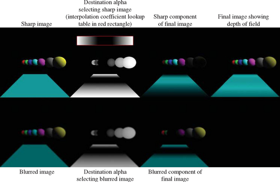
A generalization of this technique, using the programmable pipeline, renders the scene using a texture coordinate to interpolate the distance to the viewer (or focal plane) at each pixel and uses this value to look up a blurriness interpolation coefficient. This coefficient is stored in destination alpha with the rest of the scene. In subsequent passes the blurred versions of the image are created, using the techniques described previously and in Section 14.15. In the final pass a single quadrilateral the size of the window is drawn, with the orginal and blurred images bound as textures. As the quad is drawn, samples are selected from each of the bound textures and merged using the interpolation coefficient. Since the interpolation coeffecient was originally rendered to the alpha channel of the scene, it is in the alpha channel of the unblurred texture. A blurred version of the coefficient is also computed along with the RGB colors of the scene in each of the blurred texture maps. The actual blur coefficient used for interpolation is computed by averaging the unblurred and most-blurred versions of the coefficient.
If a single blurry texture is used, then a simple interpolation is done between the unblurred and blurry texture. If multiple blurrier textures are used, then the magnitude of the interpolation coefficient is used to select between two of the textures (much like LOD in mipmapping) and the samples from the two textures are interpolated.
So far, we have described how to compute the resulting image based on an interpolated bluriness coefficient, but haven’t shown how to derive the coefficient. The lens and aperture camera model described by Potmesil and Chakravarty (1981) develops a model for focus that takes into account the focal length and aperture of the lens. An in-focus point in 3D projects to a point on the image plane. A point that is out of focus maps to a circle, termed the circle of confusion, where the diameter is proportional to the distance from the plane of focus. The equation for the diameter depends on the distance from the camera to the point z, the lens focal length F, the lens aperature number n, and the focal distance (distance at which the image is in perfect focus), Zf:
Circles of diameter less than some threshold dmin are considered in focus. Circles greater than a second threshold dmax are considered out of focus and correspond to the blurriest texture. By assigning a texture coordinate with the distance from the viewer, the interpolated coordinate can be used to index an alpha texture storing the function:
This function defines the [0, 1] bluriness coefficient and is used to interpolate between the RGB values in the textures storing the original version of the scene and one or more blurred versions of the scene as previously described (Figure 12.8).
The main advantage of this scheme over a geometric scheme is that the orignal scene only needs to be rendered once. However, there are also some shortcommings. It requires fragment program support to implement the multiway interpolation, the resolution of the interpolation coefficient is limited by the bit-depth of the alpha buffer, and the fidelity is limited by the number of blurry textures used (typically 2 or 3). Some simple variations on the idea include using a fragment-program-controlled LOD bias value to alter which texture level is selected on a per-fragment basis. The c(z) value can be computed in a similar fashion and be used to control the LOD bias.
12.9 High-Dynamic Range Imaging
Conventional 8-bit per component RGB color representations can only represent two orders of magnitude in luminance range. The human eye is capable of resolving image detail spanning 4 to 5 orders of magnitude using local adaptation. The human eye, given several minutes to adjust (for example, entering a dark room and waiting), can span 9 orders of magnitude (Ward, 2001). To generate images reproducing that range requires solving two problems: enabling computations that can capture this much larger dynamic range, and mapping a high-dynamic range image to a display device with a more limited gamut.
12.9.1 Dynamic Range
One way to solve the dynamic range computation problem is to use single-precision floating-point representations for RGB color components. This can solve the problem at the cost of increased computational, storage, and bandwidth requirements. In the programmable pipeline, vertex and fragment programs support floating-point processing for all computations, although not necessarily with full IEEE-754 32-bit precision.2 While supporting single-precision floating-point computation in the pipeline is unlikely to be an issue for long, the associated storage and bandwidth requirements for 96-bit floatingpoint RGB colors as textures and color buffers can be more of an issue. There are several, more compact representations that can be used, trading off dynamic range and precision for compactness. The two most popular representations are the “half-float” and “shared-exponent” representations.
Half Float
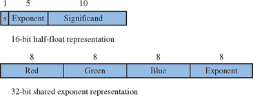
The half-float representation uses a 16-bit floating representation with 5 bits of exponent, 10 bits of significand (mantissa), and a sign bit. Like the IEEE-754 floating-point formats, normalized numbers have an implied or hidden most significant mantissa bit of 1, so the mantissa is effectively 11 bits throughout most of the range. The range of numbers that can be represented is roughly [2−16, 216] or about 10 orders of magnitude with 11 bits of precision. This representation captures the necessary dynamic range while maintaining good accuracy, at a cost of twice the storage and bandwidth of an 8-bit per-component representation. This format is seeing moderate adoption as an external image representation and rapid adoption in graphics accelerators as a texture and color buffer format.
Shared Exponent
Shared exponent representations reduce the number of bits by sharing a single exponent between all three of the RGB color components. The name RGBE is often used to describe the format. A typical representation uses a shared 8-bit exponent with three 8-bit significands for a total of 32 bits. Since the exponent is shared, the exponent from the component with largest magnitude is chosen and the mantissas of the remaining two components are scaled to match the exponent. This results in some loss of accuracy for the remaining two components if they do not have similar magnitudes to the largest component.
The RGBE representation, using 8-bit for significands and exponent, is convenient to process in an application since each element fits in a byte, but it is not an optimal distribution of the available bits for color representation. The large exponent supports a dynamic range of 76 orders of magnitude, which is much larger than necessary for color representation; the 8-bit mantissa could use more bits to retain accuracy, particularly since the least significant bits are truncated to force two of the components to match the exponent. An example of an alternative distribution of bits might include a 5-bit exponent, like the half-float representation, and a 9-bit significand (Figure 12.9).
The shared-exponent format does a good job of reducing the overall storage and bandwidth requirements. However, the extra complexity in examining a set of 3 color components, determining the exponent and adjusting the components makes the representation more expensive to generate. Furthermore, to minimize visual artifacts from truncating components the neighboring pixel values should also be examined. This extra cost results in a trend to use the representation in hardware accelerators as a read-only source format, for example, in texture maps, rather than a more general writable color buffer format.
12.9.2 Tone Mapping
Once we can represent high-dynamic range (HDR) images, we are still left with the problem of displaying them on low-dynamic range devices such as CRTs and LCD panels. One way to accomplish this is to mimic the human eye. The eye uses an adaptation process to control the range of values that can be resolved at any given time. This amounts to controlling the exposure to light, based on the incoming light intensity. This adaptation process is analogous to the exposure controls on a camera in which the size of the lens aperture and exposure times are modified to control the amount of light that passes to the film or electronic sensor.
Note that low-dynamic range displays only support two orders of magnitude of range, whereas the eye accommodates four to five orders before using adaptation. This means that great care must be used in mapping the high-dynamic range values. The default choice is to clamp the gamut range, for example, to the standard OpenGL [0, 1] range, losing all of the high-intensity and low-intensity detail. The class of techniques for mapping high-dynamic range to low-dynamic range is termed tone mapping; a specific technique is often called a tone mapping operator. Other classes of algorithms include:
1. Uniformly scaling the image gamut to fit within the display gamut, for example, by scaling about the average luminance of the image.
2. Scaling colors on a curve determined by image content, for example, using a global histogram (Ward Larson et al., 1997).
3. Scaling colors locally based on nearby spatial content. In a photographic context, this corresponds to dodging and burning to control the exposure of parts of a negative during printing (Chui et al., 1993).
Luminance Scaling
The first mapping method involves scaling about some approximation of the neutral scene luminance or key of the scene. The log-average luminance is a good approximation of this and is defined as:
The δ value is a small bias included to allow log computations of pixels with zero luminance. The log-average luminance is computed by summing the log-luminance of the pixel values of the image. This task can be approximated by sparsely sampling the image, or operating on an appropriately resampled smaller version of the image. The latter can be accomplished using texture mapping operations to reduce the image size to 64 × 64 before computing the sum of logs. If fragment programs are supported, the 64×64 image can be converted to log-luminance directly, otherwise color lookup tables can be used on the color values. The average of the 64×64 log-luminance values is also computed using successive texture mapping operations to produce 16×16, 4×4, and 1×1 images, finally computing the antilog of the 1×1 image.
The log-average luminance is used to compute a per-pixel scale factor
where a is a value between [0, 1] and represents the key of the scene, typically about 0.18. By adjusting the value of a, the linear scaling controls how the parts of the high-dynamic range image are mapped to the display. The value of a roughly models the exposure setting on a camera.
Curve Scaling
The uniform scaling operator can be converted to the non-linear operator (Reinhard, 2002)
which compresses high-luminace regions by ![]() while leaving low-luminace regions untouched. It is applied as a scale factor to the color components of each image pixel.
while leaving low-luminace regions untouched. It is applied as a scale factor to the color components of each image pixel.
It can be modified to allow high luminances to burn out:
where Lwhite is the smallest luminance value to be mapped to white. These methods preserve some detail in low-contrast areas while compressing the high luminances into a displayable range. For very high-dynamic range scenes detail is lost, leading to a need for a local tone reproduction operator that considers the range of luminance values in a local neighborhood.
Local Scaling
Local scaling emulates the photographic techniques of dodging and burning with a spatially varying operator of the form
where V is the spatially varying function evaluated over the region s. Contrast is measured at multiple scales to determine the size of the region. An example is taking the difference between two images blurred with Gaussian filters. Additional details on spatially varying operators can be found in Reinhard et al. (2002).
12.9.3 Modeling Adaptation
The adaption process of the human visual system can be simulated by varying the tone operator over time. For example, as the scene changes in response to changes to the viewer position one would normally compute a new average scene luminance value for the new scene. To model the human adaptation process, a transition is made from the current adaption level to the new scene average luminance. After a length of time in the same position the current adaption level converges to the scene average luminance value. A good choice for weighting functions is an exponential function.
12.10 Summary
This chapter describes a sampling of important image processing techniques that can be implemented using OpenGL. The techniques include a range of point-based, region-based, and geometric operations. Although it is a useful addition, the ARB imaging subset is not required for most of the techniques described here. We also examine the use of the programmable pipeline for image processing techniques and discuss some of the strengths and weaknesses of this approach. Several of the algorithms described here are used within other techniques described in later chapters. We expect that an increasing number of image processing algorithms will become im portant com ponents of other rendering algorithms.