
Antialiasing
Aliasing refers to the jagged edges and other rendering artifacts commonly associated with computer-generated images. They are caused by simplifications incorporated in various algorithms in the rendering pipeline, resulting in inaccuracies in the generated image. Usually these simplifications are necessary to create a pipeline implementation that is low in cost and capable of achieving good interactive frame rates. In this chapter we will review some of the causes of aliasing artifacts and describe some of the techniques that can be used to reduce or eliminate them.
Chapter 4 provides some of the background information regarding how images are represented digitally; the ideas behind sampling and reconstructing the spatial signals comprising an image; and some of the problems that can arise. The spatial aliasing problem appears when the sample rate of the digital image is insufficient to represent all of the high-frequency detail in the original image signal. In computer-generated or synthetic images the problem is acute because the algebraic representation of primitives can define arbitrarily high frequencies as part of an object description. One place where these occur is at the edges of objects. Here the abrupt change in the signal that occurs when crossing the edge of an object corresponds to infinitely high-frequency components. When a simple point-sampling rasterization process tries to represent these arbitrarily high frequencies, the result is aliasing artifacts.
Object edges aren’t the only place spatial aliasing artifacts appear. Aliasing artifacts are also introduced when a texture image is projected to an area that is much smaller than the original texture map. Mipmapping reduces the amount of aliasing by first creating multiple, alias-free texture images of progressively smaller sizes as a pre-processing step. During texture mapping, the projected area is used to determine the two closest texture image sizes that bracket the exact size. A new image is then created by taking a weighted sum of texels from the two images. This minimizes the more visually jarring artifacts that can appear on moving objects that are textured without using mipmapping. This aliasing problem is severe enough that mipmapping support is both defined and well-implemented in most OpenGL implementations. Antialiasing for the edges of lines, points, and polygons is also defined, but is traditionally less well supported by implementations. In particular, polygon edge antialiasing using GL_POLYGON_SMOOTH is often poorly implemented.
The simple solution to the aliasing problem is to not introduce frequency aliases during rasterization—or at least minimize them. This requires either increasing the spatial sampling rate to correctly represent the original signals, or removing the frequency components that would otherwise alias before sampling (prefiltering). Increasing the sampling rate, storing the resulting image, and reconstructing that image for display greatly increases the cost of the system. The infinitely high-frequency contributions from edge discontinuities would also imply a need for arbitrarily high sampling rates. Fortunately, the magnitude of the contribution typically decreases rapidly with increasing frequency, and these lower-magnitude, high-frequency contributions can be made much less noticeable. As a result, most of the benefit of increasing the sampling rate can be attained by increasing it by a finite amount. Despite this upper limit, it is still not very practical to double or quadruple the size of the framebuffer and enhance the display circuitry to accommodate the higher sampling rate; increasing the sampling rate alone isn’t the solution.
A second solution is to eliminate the high-frequency signal contributions before the pixel samples are created. The distortions to the image resulting from eliminating the high-frequency components, blurring, are much less objectionable compared to the distortions from aliasing. The process of eliminating the high-frequency components is referred to as band-limiting; the resulting image contains a more limited number of frequency bands. The filtering required to accomplish the band-limiting requires more computations to be performed during rasterization; depending on the specifics of the algorithm, it can be a practical addition to the rendering implementation.
10.1 Full-Scene Antialiasing
Ideally, after rendering a scene, the image should be free of aliasing artifacts. As previously described, the best way to achieve this is by eliminating as much of the aliased high-frequency information as possible while generating the pixel samples to be stored in the color buffer. First we will describe some general techniques that work on any type of primitive. Then we will describe methods that take advantage of the characteristics of polygons, lines, and points that allow them to be antialiased more effectively. Primitive-independent methods may be applied to an entire scene. Primitive-dependent methods require grouping the rendering tasks by primitive type, or choosing and configuring the appropriate antialiasing method before each primitive is drawn.
10.2 Supersampling
One popular class of antialiasing techniques samples the image at a much higher sampling rate than the color buffer resolution (for example, by a factor of 4 or 8), then postfilters these extra samples to produce the final set of pixel values. Only the postfiltered values are saved in the framebuffer; the high-resolution samples are discarded after they are filtered. This type of antialiasing method is called supersampling and the high-resolution pixels are called supersamples.1
The net effect of supersampling is to eliminate some of the high-frequency detail that would otherwise alias to low-frequency artifacts in the sample values. The process does not eliminate all of the aliasing, since the supersamples themselves contain aliased information from frequencies above the higher resolution sample rate. The aliasing artifacts from these higher frequencies are usually less noticeable, since the magnitude of the high-frequency detail does diminish rapidly as the frequency increases. There is a limit to the amount of useful supersampling. In practice, the most significant improvement comes with 4 to 16 samples; beyond that the improvements diminish rapidly.
When designing a supersampling method, the first decision to make is selecting the number of samples. After that there are two other significant choices to make: the choice of supersample locations, which we will call the sample pattern, and the method for filtering the supersamples.
The natural choice for supersample locations is a regular grid of sample points, with a spacing equal to the new sample rate. In practice, this produces poor results, particularly when using a small number of supersamples. The reason for this is that remaining aliasing artifacts from a regularly spaced sample grid tend to occur in regular patterns. These patterns are more noticable to the eye than errors with random spacings.
A remedy for this problem is to choose a more random sample pattern. This changes the high-frequency aliasing to less noticeable uncorrelated noise in the image. Methods for producing random sample patterns as described by Cook (1986) are part of a technique called stochastic supersampling. Perhaps the most useful is jittered sample patterns. They are constructed by displacing (jittering) the points on a regular super-grid with small, random displacements.
A point sample reflects the value of a single point, rather than being representative of all of the features in the pixel. Consider the case of a narrow, tall, vertical rectangle, ![]() of a pixel wide, moving horizontally from left to right across the window in 1/8th pixel steps. Using the top left sample pattern (a) shown in Figure 10.1 and the normal point sampling rules, the rectangle will alternately be sampled by the left-most two sample points, by no sample points, and then by the right-most sample points. If the same exercise is repeated using the top right sample pattern (c), at least some contribution from the rectangle will be detected more often than with sample pattern (a), since the sample points include 4 distinct x positions rather than just 2. Although this example is engineered for a vertical rectangle, it demonstrates some basic ideas for choosing better sample patterns:
of a pixel wide, moving horizontally from left to right across the window in 1/8th pixel steps. Using the top left sample pattern (a) shown in Figure 10.1 and the normal point sampling rules, the rectangle will alternately be sampled by the left-most two sample points, by no sample points, and then by the right-most sample points. If the same exercise is repeated using the top right sample pattern (c), at least some contribution from the rectangle will be detected more often than with sample pattern (a), since the sample points include 4 distinct x positions rather than just 2. Although this example is engineered for a vertical rectangle, it demonstrates some basic ideas for choosing better sample patterns:
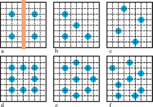
• Use a subpixel grid that is at least 4 times the sample rate in each direction.
• Choose sample points that have unique x and y coordinates.
• Include one sample point close to the center of the pixel.
A further consideration that arises when choosing sample locations is whether to use sample points beyond a pixel’s extent and into neighboring pixels. The idea of a pixel as rectangle with rigid boundaries is no more than a useful conceptual tool; there is nothing that forbids sampling outside of this region. The answer lies in the sampling and reconstruction process. Since the final pixel value results from reconstructing the signal from its supersamples, the choice of sample locations and reconstruction (postfilter) functions are intertwined. Although the results vary depending on the sample locations and filter function used, the short answer is that using overlapping supersampled regions can result in a better image.
As described in Section 4.2, a number of different low-pass filters are available to choose from to eliminate the high-frequency details. These can range from simple box or triangle filters to more computationally intensive Gaussian or other filters.
10.2.1 Supersampling by Overdrawing
A simple way to implement supersampling is to render a scene in a larger window, then postfilter the result. Although simple to implement, there are a few difficulties with this solution. One issue is that the maximum window size will limit the number of samples per-pixel, especially if the objective is to produce a large final image. The sample locations themselves use the framebuffer pixel locations, which are on a regular grid, resulting in regular patterns of aliasing artifacts.
A second problem is finding an efficient method for implementing the reconstruction filter. A simple solution is to implement the filter within the application code, but it is generally faster to use texture mapping with blending or accumulation buffer hardware as described in Section 6.3.1. Despite these limitations, the algorithm can be used effectively in many applications, particularly those where rendering time is not an issue. Some hardware accelerator vendors include this capability as an antialiasing feature that doesn’t require any changes to an existing application. Once the feature is built into the OpenGL implementation, it is often possible to support an irregular sampling pattern, further improving the antialiasing effectiveness.
10.2.2 Supersampling with the Accumulation Buffer
An approach that offers better results than overdrawing uses the accumulation buffer. It can be used very effectively to implement multipass supersampling. In each pass one supersample from the sample pattern is computed for each pixel in the scene, followed by one step of an incremental postfiltering algorithm using the accumulation buffer.
The supersamples are really just the normal pixel point samples taken at specific subpixel sample locations. The subpixel sample is generated by modifying the projection matrix with a translation corresponding to the difference between the original pixel center and the desired subpixel position. Ideally the application modifies the window coordinates by subpixel offsets directly; the most effective way to achieve this is by modifying the projection matrix. Care must be taken to compute translations to shift the scene by the appropriate amount in window coordinate space.
If a translation is multiplied onto the projection matrix stack after the projection matrix has been loaded, then the displacements need to be converted to eye coordinates. To convert a displacement in pixels to eye coordinates, multiply the displacement amount by the dimension of the eye coordinate scene, and divide by the appropriate viewport dimension:
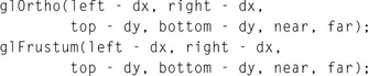
Eye coordinate displacements are incorporated into orthographic projections using glOrtho, and into perspective projections using glFrustum:
Example subpixel jitter values, organized by the number of samples needed, are taken from the OpenGL Programming Guide, and are shown in Table 10.1. (Note that some of these patterns are a little more regular horizontally and vertically than is optimal.)
Table 10.1
| Count | Values |
| 2 | {0.25, 0.75}, {0.75, 0.25} |
| 3 | {0.5033922635, 0.8317967229}, {0.7806016275, 0.2504380877}, {0.2261828938, 0.4131 553612} |
| 4 | {0.375, 0.25}, {0.125, 0.75}, {0.875, 0.25}, {0.625, 0.75} |
| 5 | {0.5, 0.5}, {0.3, 0.1}, {0.7, 0.9}, {0.9, 0.3}, {0.1, 0.7} |
| 6 | {0.4646464646, 0.4646464646}, {0.1313131313, 0.7979797979}, {0.5353535353, 0.8686868686}, {0.8686868686, 0.5353535353}, {0.7979797979, 0.1313131313}, {0.2020202020, 0.2020202020} |
| 8 | {0.5625, 0.4375}, {0.0625, 0.9375}, {0.3125, 0.6875}, {0.6875, 0.8125}, {0.8125, 0.1875}, {0.9375, 0.5625}, {0.4375, 0.0625}, {0.1875, 0.3125} |
| 9 | {0.5, 0.5}, {0.1666666666, 0.9444444444}, {0.5, 0.1666666666}, {0.5, 0.8333333333}, {0.1666666666, 0.2777777777}, {0.8333333333, 0.3888888888}, {0.1666666666, 0.61 11 11 111 1}, {0.8333333333, 0.7222222222}, {0.8333333333, 0.0555555555} |
| 12 | {0.4166666666, 0.625}, {0.9166666666, 0.875}, {0.25, 0.375}, {0.4166666666, 0.125}, {0.75, 0.125}, {0.0833333333, 0.125}, {0.75, 0.625}, {0.25, 0.875}, {0.5833333333, 0.375}, {0.9166666666, 0.375}, {0.0833333333, 0.625}, {0.583333333, 0.875} |
| 16 | {0.375, 0.4375}, {0.625, 0.0625}, {0.875, 0.1875}, {0.125, 0.0625}, {0.375, 0.6875}, {0.875, 0.4375}, {0.625, 0.5625}, {0.375, 0.9375}, {0.625, 0.3125}, {0.125, 0.5625}, {0.125, 0.8125}, {0.375, 0.1875}, {0.875, 0.9375}, {0.875, 0.6875}, {0.125, 0.3125}, {0.625, 0.8125} |
The reconstruction filter is defined by the sample locations and the scale factor used in each accumulation operation. A box filter is implemented by accumulating each image with a scale factor equal to 1/n, where n is the number of supersample passes. More sophisticated filters are implemented by using different weights for each sample location.
Using the accumulation buffer, it is easy to make trade-offs between quality and speed. For higher quality images, simply increase the number of scenes that are accumulated. Although it is simple to antialias the scene using the accumulation buffer, it is much more computationally intensive and probably slower than the more specific antialiasing algorithms that are described next.
10.2.3 Multisample Antialiasing
Multisampling is a form of single-pass supersampling that is directly supported in OpenGL.2 When using hardware with this support, multisampling produces high-quality results with less performance overhead, and requires minimal changes to an existing application. It was originally available as an OpenGL extension and later added to the core specification in version 1.3. The multisampling specification largely defines a set of rules for adding supersampling to the rendering pipeline. The number of samples can vary from implementation to implementation, but typically ranges between 2 and 8.
Each pixel fragment is extended to include a fixed number of additional texture coordinates and color, depth, and stencil values. These sample values are stored in an extra buffer called the multisample buffer. The regular color buffer continues to exist and contains the resolved color—the postfiltered result. There are no equivalent resolved depth and stencil buffers however; all depth and stencil values are part of the multisample buffer. It is less useful to compute postfiltered depth or stencil results since they are typically used for resolving visible surfaces, whereas the resolved color is used for display. Some implementations may defer computation of the resolved color values until the multisample buffer is read for display or the color buffer is used as a source in another OpenGL operation, for example, glReadPixels. For the most part, multisampling doesn’t change the operation of the rendering pipeline, except that each pipeline step operates on each sample in the fragment individually.
A multisample fragment also differs from a non-multisample fragment because it contains a bitmask value termed coverage. Each bit in the mask corresponds to a sample location. The value of the bit indicates whether the primitive fragment intersects (covers) that sample point. One way to think of the coverage value is as a mask indicating which samples in the fragment correspond to part of the primitive and which do not. Those that are not part of the primitive can be ignored in most of the pipeline processing. There are many ways to make a multisample implementation more efficient. For example, the same color value or texture coordinate may be used for all samples within a fragment. The multisample buffer may store its contents with some form of compression to reduce space requirements. For example, the multisample buffer contents may be encoded so as to exploit coherence between samples within a pixel.
The OpenGL specification does not define the sample locations and they are not queriable by the application. The sample points may extend outside a pixel and the locations may vary from pixel to pixel. This latter allowance makes it possible to implement some form of stochastic sampling, but it also breaks the invariance rules, since the values computed for a fragment are dependent on the pixel location.
As described in Section 6.1, implementations often use the same color and texture coordinate values at all sample locations. This affords a substantial performance improvement over true supersampling since color and texture coordinate values are evaluated once per-pixel and the amount of data associated with a fragment is greatly reduced. However, distinct depth and stencil values are maintained for each sample location to ensure that the edges of interpenetrating primitives are resolved correctly. A disadvantage of this optimization is that interior portions of primitives may still show aliasing artifacts. This problem becomes more apparent with the use of complex per-fragment shading computations in fragment programs. If the fragment program doesn’t filter the results of the shading calculations, then aliasing artifacts may result.
Generally, multisampling provides a good full-scene (edge) antialiasing solution. Most importantly, to use it only requires turning it on; other than that, there are no changes required of the application. Using multisampling can be completely automatic. If the application selects a multisample-capable framebuffer configuration, multisampling is enabled by default. The OpenGL implementation pays the cost of extra storage for the the multisample buffer and additional per-sample processing at each fragment, but this cost will be reduced over time with advances in the state of the art. Some implementations may even combine multisampling with the brute force overdraw supersampling technique to further increase the effective sampling rate. Unfortunately, supersampling with a small number of samples (less than 16) is not an antialiasing panacea. By contrast, film-quality software renderers often use supersampling with considerably larger numbers of samples, relying on adaptive sampling techniques to determine the number of samples required within each pixel to reduce the computational requirements.
While supersampling with a small number of samples may produce good results, the results for point and line primitives using primitive-specific methods may be substantially better. Fortunately, these other techniques can be used in concert with multisampling.
10.2.4 Drawbacks
In some cases, the ability to automatically antialias the images rendered by an application can be a drawback. Taking advantage of the flexibility of the approach, some hardware vendors have provided methods for turning on full scene antialiasing without requiring any support from the application. In some cases, this can cause problems for an application not designed to be used with antialiasing.
For example, an application may use bitmapped fonts to display information to the viewer. Quite often, this text will show artifacts if full scene antialiasing is applied to it, especially if the text is moved across the screen. Sampling errors will make the text appear “blotchy”; if the text is small enough, it can become unreadable. Since most antialiasing implementations filter samples in different ways, it can be difficult for the application developer to correct for this on all hardware. In the end, full scene antialiasing is not always appropriate. Care must be taken to understand an application’s display techniques before turning it on.
10.3 Area Sampling
Another class of antialiasing algorithms uses a technique called area sampling. The idea behind area sampling is that the value of a pixel sample should be proportional to the area of the pixel intersected by the primitive. This is in contrast to point sampling and supersampling which derive a pixel value from the intensity of the primitive at one or more infinitely small sample points. With area sampling, the contribution from a primitive partially overlapping a pixel is always accounted for. In contrast, a point-sampled primitive makes no contribution to a pixel if it doesn’t overlap a sample point.
Mathematically, area sampling is equivalent to sampling at infinitely many points followed by filtering. The choice of point locations and filter types leads to several variations of area sampling. The simplest form, called unweighted area sampling, uses a box filter to produce an average of the samples. A disadvantage of unweighted area sampling is that moving objects can still generate pixel flicker, since a pixel sample can change abruptly as a primitive moves in and out of the area associated with the pixel (as illustrated in Figure 10.2). The flicker can be corrected by overlapping sample areas with adjacent pixels. The contributions from the neighboring pixels are given a lower weight than contributions from within the pixel. This type of sampling is called weighted area sampling. It is similar to using a supersampling approach that includes some supersamples outside of the pixel followed by a triangle or Gaussian low-pass filter to perform the reconstruction.
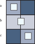
Figure 10.2 Flicker artifacts with unweighted area sampling. A bright fragment 1/4th of a pixel in size moves horizontally across the screen in successive rows.
One of the main difficulties with area sampling techniques is computing the correct result when multiple primitives overlap the same pixel. If two primitives overlap different parts of the pixel, then both should contribute to it. The pixel then becomes the area-weighted sum of the two primitive colors. If part of one primitive is occluded by the other primitive, then the correct approach becomes more complicated. Only the visible parts of two overlapping primitives should contribute. Therein lies the problem—correctly combining visible surface determination with area computations. The supersampling algorithms described previously work correctly and automatically for interpenetrating surfaces since each supersample is correctly depth-buffered before postfiltering. To render an image correctly using area sampling, the visible surface and area sampling processing must be performed together so that the weighted areas for the visible parts of each primitive within each pixel can be computed correctly.
The processing implications of this approach can be severe. It requires that the visible part of each primitive overlapping a pixel must be computed before the area can be determined. There are several algorithms for doing this (Catmill, 1978; Carpenter, 1984); typically one row of pixels (a scan line) or a small rectangular area of pixels, called a tile, are processed one at a time. All primitives that intersect a pixel row or tile are processed together. Fragments are computed at each pixel for each primitive, the fragments are depth-sorted, and the visible areas of each fragment are determined. The normalized areas are then used to compute the weighted sum of fragment colors to produce the pixel color. The mathematically correct algorithm clips each fragment against every other fragment in the pixel and sorts the results from front to back. Other algorithms trade off the pixel-level clipping cost for approximations of coverage, using a supersampling-like subpixel grid to track which parts of a pixel a fragment covers while retaining the area-based color value.
In general, adding such an algorithm to the OpenGL pipeline requires considerable effort. To implement the visible surface algorithm, the entire scene must be buffered within the pipeline. Multipass algorithms become more complicated if the combined results need to be antialiased. There is no depth buffer, since a different visible surface algorithm is used. This requires reformulation of techniques that use the stencil and depth buffers.
Nevertheless, the area sampling ideas are quite useful when applied in more specific circumstances. Good candidates for this approach are antialiased lines and points. Their area coverage is easier to compute analytically and the correctness of hidden surface resolution is not as critical as it is for polygons.
10.4 Line and Point Antialiasing
Line and point antialiasing are often considered separately from polygon antialiasing, since there are additional techniques that can be used specifically for these simpler primitives. For certain applications, such as computer-aided design programs, line rendering is pervasive enough that it is worth having special purpose hardware to improve the rendering quality.
Mathematically, a line is infinitely thin. Attempting to compute the percentage of a pixel covered by an infinitely thin object would result in no coverage, so generally one of the following two methods is used:
1. The line is modeled as a long, thin, single-pixel-wide quadrilateral. Area sampling computes the percentage of pixel coverage for each pixel touching the line and this coverage percentage is used as an alpha value for blending.
2. The line is modeled as an infinitely thin transparent glowing object. This method treats a line as if it were drawn on a vector stroke display; these displays draw lines by deflecting the electron beam along the length of the line. This approach requires the implementation to compute the effective shape of a simulated beam that moves across the CRT phosphors.
OpenGL has built-in support for antialiasing lines and points, selected by enabling GL_POINT_SMOOTH or GL_LINE_SMOOTH. Quality hints are provided using glHint. The hint parameter can be GL_FASTEST to indicate that the most efficient option should be chosen, GL_NICEST to indicate the highest quality option should be chosen, or GL_DONT_CARE to indicate no preference.
When antialiasing is enabled, OpenGL computes an alpha value representing either the fraction of each pixel that is covered by the line or point or the beam intensity for the pixel as a function of the distance of the pixel center from the line center. The setting of the GL_LINE_SMOOTH and the GL_POINT_SMOOTH hints determines the accuracy of the calculation used when rendering lines and points, respectively. When the hint is set to GL_NICEST, a larger filter footprint may be applied, causing more fragments to be generated and rendering to run more slowly.
Regardless of which line antialiasing method is used in a particular implementation of OpenGL, it can be approximated by choosing the right blend equation. The critical insight is realizing that antialiased lines and points are a form of transparent primitive (see Section 11.8). This requires blending to be enabled so that each incoming pixel fragment will be combined with the value already in the framebuffer, controlled by the alpha value.
The best approximation of a one-pixel-wide quadrilateral is achieved by setting the blending factors to GL_SRC_ALPHA (source) and GL_ONE_MINUS_SRC_ALPHA (destination). To best approximate the lines of a stroke display, use GL_ONE for the destination factor. Note that this second blend equation only works well on a black background and does not produce good results when drawn over bright objects.
As with all transparent primitives, antialiased lines and points should not be drawn until all opaque objects have been drawn first. Depth buffer testing remains enabled, but depth buffer updating is disabled using glDepthMask(GL_FALSE). This allows the antialiased lines and points to be occluded by opaque objects, but not by one another. Antialiased lines drawn with full depth buffering enabled produce incorrect line crossings and can result in significantly worse rendering artifacts than with antialiasing disabled. This is especially true when many lines are drawn close together.
Setting the destination blend mode to GL_ONE_MINUS_SRC_ALPHA may result in order-dependent rendering artifacts if the antialiased primitives are not drawn in back to front order. There are no order-dependent problems when using a setting of GL_ONE, however. Pick the method that best suits the application.
Incorrect monitor gamma settings are much more likely to become apparent with antialiased lines than with shaded polygons. Gamma should typically be set to 2.2, but some workstation manufacturers use values as low as 1.6 to enhance the perceived contrast of rendered images. This results in a noticable intensity nonlinearity in displayed images. Signs of insufficient gamma are “roping” of lines and moire patterns where many lines come together. Too large a gamma value produces a “washed out” appearance. Gamma correction is described in more detail in Section 3.1.2.
Antialiasing in color index mode can be tricky. A correct color map must be loaded to get primitive edges to blend with the background color. When antialiasing is enabled, the last four bits of the color index indicate the coverage value. Thus, 16 contiguous color map locations are needed, containing a color ramp ranging from the background color to the object’s color. This technique only works well when drawing wireframe images, where the lines and points typically are blended with a constant background. If the lines and/or points need to be blended with background polygons or images, RGBA rendering should be used.
10.5 Antialiasing with Textures
Points and lines can also be antialiased using the filtering provided by texturing by using texture maps containing only alpha components. The texture is an image of a circle starting with alpha values of one at the center and rolling off to zero from the center to the edge. The alpha texel values are used to blend the point or rectangle fragments with the pixel values already in the framebuffer. For example, to draw an antialiased point, create a texture image containing a filled circle with a smooth (antialiased) boundary. Then draw a textured polygon at the point location making sure that the center of the texture is aligned with the point’s coordinates and using the texture environment GL_MODULATE. This method has the advantage that a different point shape may be accommodated by varying the texture image.
A similar technique can be used to draw antialiased line segments of any width. The texture image is a filtered line. Instead of a line segment, a texture-mapped rectangle, whose width is the desired line width, is drawn centered on and aligned with the line segment. If line segments with squared ends are desired, these can be created by using a one dimensional texture map aligned across the width of the rectangle polygon.
This method can work well if there isn’t a large disparity between the size of the texture map and the window-space size of the polygon. In essence, the texture image serves as a pre-filtered, supersampled version of the desired point or line image. This means that the roll-off function used to generate the image is a filtering function and the image can be generated by filtering a constant intensity line, circle or rectangle. The texture mapping operation serves as a reconstruction filter and the quality of the reconstruction is determined by the choice of texture filter. This technique is further generalized to the concept of texture brushes in Section 19.9.
10.6 Polygon Antialiasing
Antialiasing the edges of filled polygons using area sampling is similar to antialiasing points and lines. Unlike points and lines, however, antialiasing polygons in color index mode isn’t practical. Object intersections are more prevalent, and OpenGL blending is usually necessary to get acceptable results.
As with lines and points, OpenGL has built-in support for polygon antialiasing. It is enabled using glEnable with GL_POLYGON_SMOOTH. This causes pixels on the edges of the polygon to be assigned fractional alpha values based on their pixel coverage. The quality of the coverage values are controlled with GL_POLYGON_SMOOTH_HINT.
As described in Section 10.3, combined area sampling and visibility processing is a difficult problem. In OpenGL an approximation is used. To make it work, the application is responsible for part of the visibility algorithm by sorting the polygons from front to back in eye space and submitting them in that order. This antialiasing method does not work without sorting. The remaining part of resolving visible surfaces is accomplished using blending. Before rendering, depth testing is disabled and blending is enabled with the blending factors GL_SRC_ALPHA_SATURATE (source) and GL_ONE (destination). The final color is the sum of the destination color and the scaled source color; the scale factor is the smaller of either the incoming source alpha value or one minus the destination alpha value. This means that for a pixel with a large alpha value, successive incoming pixels have little effect on the final color because one minus the destination alpha is almost zero.
At first glance, the blending function seems a little unusual. Section 11.1.2 describes an algorithm for doing front-to-back compositing which uses a different set of blending factors. The polygon antialiasing algorithm uses the saturate source factor to ensure that surfaces that are stitched together from multiple polygons have the correct appearance. Consider a pixel that lies on the shared edge of two adjacent, opaque, visible polygons sharing the same constant color. If the two polygons together cover the entire pixel, then the pixel color should be the polygon color. Since one of the fragments is drawn first, it will contribute the value α1C. When the second contributing fragment is drawn, it has alpha value α2. Regardless of whether α1 or α2 is larger, the resulting blended color will be α1C + (1 − α1) C = C, since the two fragments together cover the entire pixel α2 = 1 − α1.
Conversely, if the fragments are blended using a traditional compositing equation, the result is α1C + (1 − α1)α2C + (1 − α1)(1 − α2)Cbackground and some of the background color “leaks” through the shared edge. The background leaks through because the second fragment is weighted by (1 − α1)α2. Compare this to the first method that uses either α2 or (1 − α1), whichever is smaller (in this case they are equal). This blending equation ensures that shared edges do not have noticable blending artifacts and it still does a reasonable job of weighting each fragment contribution by its coverage, giving priority to the fragments closest to the eye. More details regarding this antialiasing formula versus the other functions that are available are described in Section 11.1.2. It useful to note that A-buffer-related algorithms avoid this problem by tracking which parts of the pixel are covered by each fragment, while compositing does not.
Since the accumulated coverage is stored in the color buffer, the buffer must be able to store an alpha value for every pixel. This capability is called “destination alpha,” and is required for this algorithm to work. To get a framebuffer with destination alpha, you must request a visual or pixel format that has it. OpenGL conformance does not require implementations to support a destination alpha buffer so an attempt to select this visual may not succeed.
This antialiasing technique is often poorly supported by OpenGL implementations, since the edge coverage values require extra computations and destination alpha is required. Implementations that support multisample antialiasing can usually translate the coverage mask into an alpha coverage value providing a low-resolution version of the real coverage. The algorithm also doesn’t see much adoption since it places the sorting burden on the application. However, it can provide very good antialiasing results; it is often used by quality-driven applications creating “presentation graphics” for slide shows and printing.
A variant polygon antialiasing algorithm that is frequently tried is outlining non-antialiased polygons with antialiased lines. The goal is to soften the edges of the polygons using the antialiased lines. In some applications it can be effective, but the results are often of mixed quality since the polygon edges and lines are not guaranteed to rasterize to the same set of pixel locations.
10.7 Temporal Antialiasing
Thus far, the focus has been on aliasing problems and remedies in the spatial domain. Similar sampling problems also exist in the time domain. When an animation sequence is rendered, each frame in the sequence represents a point in time. The positions of moving objects are point-sampled at each frame; the animation frame rate defines the sampling rate. An aliasing problem analogous to the spatial aliasing occurs when object positions are changing rapidly and the motion sampling rate is too low to correctly capture the changes. This produces the familiar strobe-like temporal aliasing artifacts, such as vehicle wheels appearing to spin more slowly than they should or even spinning backward. Similar to pixel colors and attributes, the motion of each object can be thought of as a signal, but in the time domain instead of the spatial one. These time domain signals also have corresponding frequency domain representations; aliasing artifacts occur when the high-frequency parts of the signal alias to lower frequency signals during signal reconstruction.
The solutions for temporal aliasing are similar to those for spatial aliasing; the sampling rate is increased to represent the highest frequency present, or the high-frequency components are filtered out before sampling. Increasing the sampling rate alone isn’t practical, since the reconstruction and display process is typically limited to the video refresh rate, usually ranging between 30Hz and 120Hz. Therefore, some form of filtering during sampling is used. The result of the filtering process is similar to the results achieved in cinematography. When filming, during the time period when the shutter is held open to expose the film, the motion of each object for the entire exposure period is captured. This results in the film integrating an infinite number of time sample points over the exposure time. This is analogous to performing a weighted average of point samples. As with supersampling, there are quality vs. computation trade-offs in the choice of filter function and number of sample points.
10.7.1 Motion Blur
The idea of generating a weighted average of a number of time samples from an animation is called motion blur. It gets this name from the blurry image resulting from averaging together several samples of a moving object, just as a camera with too low of a shutter speed captures a blurred image of a moving object.
One simple way to implement motion blur is with the accumulation buffer. If the display rate for an animation sequence is 30 frames per second and we wish to include 10 temporal samples for each frame, then the samples for time t seconds are generated from the sequence of frames computed at t−5x, t−4x, t−3x, …, t, t + 1x, t + 2x, … t + 4x, where ![]() . These samples are accumulated with a scale of
. These samples are accumulated with a scale of ![]() to apply a box filter. As with spatial filtering, the sample sets for each frame may overlap to create a better low-pass filter, but typically this is not necessary.
to apply a box filter. As with spatial filtering, the sample sets for each frame may overlap to create a better low-pass filter, but typically this is not necessary.
For scenes in which the moving objects are in front of the static ones, an optimization can be performed. Only the objects that are moving need to be re-rendered at each sample. All of the static objects are rendered and accumulated with full weight, then the objects that are moving are drawn at each time sample and accumulated. For a single moving object, the steps are:
1. Render the scene without the moving object, using glAccum(GL_LOAD, 1.0f).
2. Accumulate the scene n times, with the moving object drawn against a black background, using glAccum(GL_ACCUM, 1.0f/n).
3. Copy the result back to the color buffer using glAccum(GL_RETURN, 1.0f).
This optimization is only correct if the static parts of the scene are completely unchanging. If depth buffering is used, the visible parts of static objects may change as the amount of occlusion by moving objects changes. A different optimization is to store the contents of the color and depth buffer for the static scene in a pbuffer and then restore the buffers before drawing the moving objects for each sample. Of course, this optimization can only improve performance if the time to restore the buffers is small relative to the amount of time it takes to draw the static parts of the scene.
The filter function can also be altered empirically to affect the perceived motion. For example, objects can be made to appear to accelerate or decelerate by varying the weight for each accumulation. If the weights are sequentially decreased for an object, then the object appears to accelerate. The object appears to travel further in later samples. Similarly, if the weights are increased, the object appears to decelerate.
10.8 Summary
In this chapter we reviewed supersampling and area sampling spatial antialiasing methods and how they are supported in the OpenGL pipeline. We also described temporal antialiasing for animation, and its relationship to spatial antialiasing.
In the next chapter we look at how blending, com positing, and transparency are supported in the pipeline. These ideas and algorithms are interrelated: they overlap with some of the algorithms and ideas described for area sampling-based antialiasing.