Illustration and Artistic Techniques
In applications such as scientific visualization and technical illustration, photorealism detracts from rather than enhances the information in the rendered image. Applications such as cartography and CAD benefit from the use of hidden surface elimination and 3D illumination and shading techniques, but the goal of increased insight from the generated images suggests some different processing compared to those used to achieve photorealism.
Strict use of photorealistic models and techniques also hampers applications striving to provide greater artistic freedom in creating images. Examples of such applications including digital image enhancement, painting programs, and cartoon-rendering applications. One aspect often shared by such applications is the use of techniques that emulate traditional modeling, lighting, and shading processes. Some examples of traditional processes are paint brush strokes and charcoal drawing.
19.1 Projections for Illustration
Traditional perspective projection models the optical effect of receding lines converging at a single point on the horizon, called the vanishing point. Outside the computer graphics field, perspective projections are called linear perspective projections. Linear perspective is the ideal model for reproducing a real-world scene the way it would be captured by a camera lens or a human eye. In some technical applications, such as architectural presentations, linear perspective serves the needs of the viewer well. In other technical applications, (however, such as engineering and mechanical design) parallel projections prove more useful. With parallel projections, edges that are parallel in 3D space remain parallel in the 2D projection. Parallel projections have many properties that make them useful for both engineering and artistic applications.
In engineering applications, it is desirable to avoid distorting the true geometry of the object, allowing measurements to be taken directly from the drawing. In the simplest forms of engineering drawings, a single view of the object is generated (such as a front-, top-, or right-side view). These individual views can be combined to create a multiview projection. Alternatively, drawings can be created that show more than one face of an object simultaneously, providing a better sense of the object. Such drawings are generally referred to as projections, since they are generated from a projection in which the object is aligned in a canonical position with faces parallel to the coordinate planes. Using this nomenclature, the drawing is defined by the position and orientation of the viewing (projection) plane, and the lines of sight from the observer to this plane.
Several types of projections have been in use for engineering drawings since the nineteenth century. These projections can be divided into two major categories: axonometric and oblique projections.
19.1.1 Axonometric Projection
Orthographic projections are parallel projections in which the lines of sight are perpendicular to the projection plane. The simplest orthographic projections align the projection plane so that it is perpendicular to one of the coordinate axis. The OpenGL glOrtho command creates an orthographic projection where the projection plane is perpendicular to the z axis. This orthographic projection shows the front elevation view of an object. Moving the projection plane so that it is perpendicular to the x axis creates a side elevation view, whereas moving the projection plane to be perpendicular to the y axis produces a top or plan view. These projections are most easily accomplished in the OpenGL pipeline using the modelview transformation to change the viewing direction to be parallel to the appropriate coordinate axis.
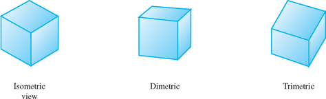
Axonometric projections are a more general class of orthographic projections in which the viewing plane is not perpendicular to any of the coordinate axes. Parallel lines in the 3D object continue to remain parallel in the projection, but lines are foreshortened and angles are not preserved. Axonometric projections are divided into three classes according to the relative foreshortening of lines parallel to the coordinate axis.
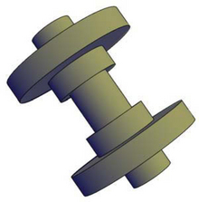
Isometric projection is the most frequently used axonometric projection for engineering drawings. Isometric projection preserves the relative lengths of lines parallel to all three of the coordinate axes and projects the coordinate axes to lines that are 60 degrees apart. An isometric projection corresponds to a viewing plane oriented such that the normal vector has all three components equal, ![]() . Object edges that are parallel to the coordinate axes are shortened by 0.8165. The y axis remains vertical, and the x and z axes make 30-degree angles with the horizon, as shown in Figure 19.1. To allow easier direct measurement, isometric projections are sometimes scaled to compensate for the foreshortening to produce an isometric drawing rather than an isometric projection.
. Object edges that are parallel to the coordinate axes are shortened by 0.8165. The y axis remains vertical, and the x and z axes make 30-degree angles with the horizon, as shown in Figure 19.1. To allow easier direct measurement, isometric projections are sometimes scaled to compensate for the foreshortening to produce an isometric drawing rather than an isometric projection.
An isometric projection is generated in OpenGL by transforming the viewing plane followed by an orthographic projection. The viewing plane transformation can be computed using gluLookAt, setting the eye at the origin and the look-at point at (−1, −1, −1)1 or one of the seven other isometric directions.
Equal foreshortening along all three axes results in a somewhat unrealistic looking appearance. This can be alleviated in a controlled way, by increasing or decreasing the foreshortening along one of the axes. A dimetric projection foreshortens equally along two of the coordinate axes by constraining the magnitude of two of the components of the projection plane normal to be equal. Again, gluLookAt can be used to compute the viewing transformation, this time maintaining the same component magnitude for two of the look-at coordinates and choosing the third to improve realism. Carefully choosing the amount of foreshortening can still allow direct measurements to be taken along all three axes in the resulting drawing.
Trimetric projections have unequal foreshortening along all of the coordinate axes. The remaining axonometric projections fall into this category. Trimetric projections are seldom used in technical drawings.
19.1.2 Oblique Projection
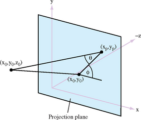
An oblique projection is a parallel projection in which the lines of sight are not perpendicular to the projection plane. Commonly used oblique projections orient the projection plane to be perpendicular to a coordinate axis, while moving the lines of sight to intersect two additional sides of the object. The result is that the projection preserves the lengths and angles for object faces parallel to the plane. Oblique projections can be useful for objects with curves if those faces are oriented parallel to the projection plane.
To derive an oblique projection, consider the point (x0, y0, Z0) projected to the position (xp, yp) (see Figure 19.2). The projectors are defined by the two angles: θ and φ, θ is the angle between the line L =[(x0, y0), (xp, yp)] and the projection plane, φ is the angle between the line L and the x axis. Setting l = ![]() L
L![]() /z0 = 1/tan θ, the general form of the oblique projection is
/z0 = 1/tan θ, the general form of the oblique projection is
For an orthographic projection, the projector is perpendicular and the length of the line L is zero, reducing the projection matrix to the identity. Two commonly used oblique projections are the cavalier and cabinet projections. The cavalier projection preserves the lengths of lines that are perpendicular or parallel to the projection plane, with lines of sight at θ = φ = 45 degrees. However, the fact that length is preserved for perpendicular lines gives rise to an optical illusion where perpendicular lines look longer than their actual length, since the human eye is used to compensating for perspective foreshortening. To correct for this, the cabinet projection shortens lines that are perpendicular to the projection plane to one-half the length of parallel lines and changes the angle θ to atan(2) = 63.43 degrees.
To use an oblique projection in the OpenGL pipeline, the projection matrix P is computed and combined with the matrix computed from the glOrtho command. Matrix P is used to compute the projection transformation, while the orthographic matrix provides the remainder of the view volume definition. The P matrix assumes that the projection plane is perpendicular to the z axis. An additional transformation can be applied to transform the viewing direction before the projection is applied.
19.2 Nonphotorealistic Lighting Models
Traditional technical illustration practices also include methods for lighting and shading. These algorithms are designed to improve clarity rather than embrace photorealism. In Gooch (1998, 1999), lighting and shading algorithms are developed based on traditional technical illustration practices. These practices include the following.
• Use of strong edge outlines to indicate surface boundaries, silhouette edges, and discontinuities.
• Matte objects are shaded with a single light source, avoiding extreme intensities and using hue to indicate surface slope.
• Metal objects are shaded with exaggerated anisotropic reflection.
Nonphotorealistic lighting models for both matte and metal surfaces are described here.
19.2.1 Matte Surfaces
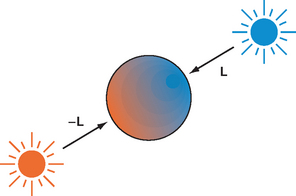
The model for matte surfaces uses both luminance and hue changes to indicate surface orientation. This lighting model reduces the dynamic range of the luminance, reserving luminance extremes to emphasize edges and highlights. To compensate for the reduced dynamic range and provide additional shape cues, tone-based shading adds hue shifts to the lighting model. Exploiting the perception that cool colors (blue, violet, green) recede from the viewer and warm colors (red, orange, yellow) advance, a sense of depth is added by including cool-to-warm color transitions in the model. The diffuse cosine term is replaced with the term
where ![]() and
and ![]() are linear combinations of a cool color (a shade of blue) combined with the object’s diffuse reflectance, and a warm color (yellow) combined with the object’s diffuse reflectance. A typical value for
are linear combinations of a cool color (a shade of blue) combined with the object’s diffuse reflectance, and a warm color (yellow) combined with the object’s diffuse reflectance. A typical value for ![]() is (0., 0., .4) + .2dm and for
is (0., 0., .4) + .2dm and for ![]() is (.4, .4, 0.) + .6dm. The modified equation uses a cosine term that varies from [−1, 1] rather than clamping to [0, 1].
is (.4, .4, 0.) + .6dm. The modified equation uses a cosine term that varies from [−1, 1] rather than clamping to [0, 1].
If vertex programs are not supported, this modified diffuse lighting model can be approximated using fixed-function OpenGL lighting using two opposing lights (L, − L), as shown in Figure 19.3. The two opposing lights are used to divide the cosine term range in two, covering the range [0, 1] and [−1, 0] separately. The diffuse intensities are set to ![]() and
and ![]() respectively, the ambient intensity is set to
respectively, the ambient intensity is set to ![]() and the specular intensity contribution is set to zero. Objects are drawn with the material reflectance components set to one (white).
and the specular intensity contribution is set to zero. Objects are drawn with the material reflectance components set to one (white).
Highlights can be added in a subsequent pass using blending to accumulate the result. Alternatively, the environment mapping techniques discussed in Section 15.9 can be used to capture and apply the BRDF at the expensive of computing an environment map for each different object material.
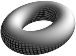
19.2.2 Metallic Surfaces
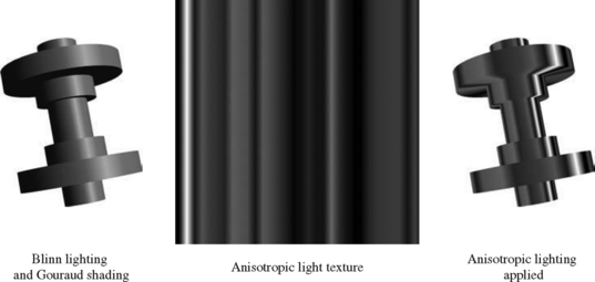
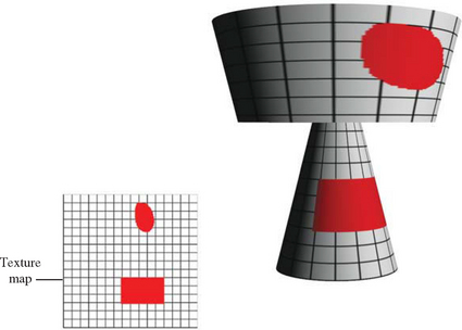
For metallic surfaces, the lighting model is further augmented to simulate the appearance of anisotropic reflection (Section 15.9.3). While anisotropic reflection typically occurs on machined (milled) metal parts rather than polished parts, the anisotropic model is still used to provide a cue that the surfaces are metal and to provide a sense of curvature. To simulate the anisotropic reflection pattern, the curved surface is shaded with stripes along the parametric axis of maximum curvature. The intensity of the stripes are random values between 0.0 and 0.5, except the stripe closest to the light source, which is set to 1.0, simulating a highlight. The values between the stripes are interpolated. This process is implemented in the OpenGL pipeline using texture mapping. A small 1D or 2D luminance texture is created containing the randomized set of stripe values. The stripe at s coordinate zero (or some well-known position) is set to the value 1. The object is drawn with texture enabled, the wrap mode set to GL_CLAMP, and the s texture coordinate set to vary along the curvature. The position of the highlight is adjusted by biasing the s coordinate with the texture matrix. This procedure is illustrated in Figure 19.4.
19.3 Edge Lines
An important aspect of the lighting model is reducing the dynamic range of the luminance to make edges and highlights more distinct. Edges can be further emphasized by outlining the silhouette and boundary edges in a dark color (see Figure 19.5). Algorithms for drawing silhouette lines are described in Section 16.7.4. Additional algorithms using image-processing techniques, described in Saito (1990) can be implemented using the OpenGL pipeline (as described in Chapter 12). Gooch (1999) and Markosian (1997) discuss software methods for extracting silhouette edges that can then be drawn as lines.
19.4 Cutaway Views
Engineering drawings of complex objects may show a cutaway view, which removes one or more surface layers of the object (shells) to reveal the object’s inner structure. A simple way to accomplish this is to not draw the polygons comprising the outer surfaces. This shows inner detail, but also removes the information relating the inner structure to the outer structure. To restore the outer detail, the application may draw part of the outer surface, discarding polygons only in one part of the surface where the inner detail should show through. This requires the application to classify the surface polygons into those to be drawn and those to be discarded. The resulting hole created in the surface will not have a smooth boundary.
Alternatively, clip planes can be used to create cross-sectional views by discarding surface geometry in one of the half-spaces defined by the clip plane. Multiple clip planes can be used in concert to define more complex culling regions. Reintroducing the clipped polygons into the drawing as partially transparent surfaces provides some additional context for the drawing.
Another method for using transparency is to draw the outer surface while varying the surface transparency with the distance from the viewer. Polygons that are most distant from the viewer are opaque, while polygons closest to the viewer are transparent, as shown in Figure 19.6. Seams or significant boundary edges within the outer shell may also be included by drawing them with transparency using a different fading rate than the shell surface polygons.
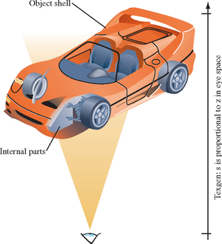
This technique uses OpenGL texture mapping and texture coordinate generation to vary the alpha component of the object shell. The object is divided into two parts that are rendered separately: the shell polygons and the interior polygons. First, the depth-buffered interior surfaces are drawn normally. Next, the object shell is rendered using a 1D texture map containing an alpha ramp, to replace the alpha component of each polygon fragment. Texture coordinate generation is used to create an s coordinate that increases with the distance of the vertex along the −z axis. The shell surface is rendered using the alpha-blending transparency techniques described in Section 11.8. The edges of the shell are rendered in a third pass, using a slightly different 1D texture map or texture generation plane equation to produce a rate of transparency change that differs from that of the shell surface.
1. Draw the object internals with depth buffering.
2. Enable and configure a 1D texture ramp using GL_ALPHA as the format and GL_REPLACE as the environment function.
3. Enable and configure eye-linear texture coordinate generation for the s component, and set the s eye plane to map −z over the range of the object shell cutaway from 0 to 1.
4. Disable depth buffer updates and enable blending, setting the source and destination factors to GL_SRC_ALPHA and GL_ONE_MINUS_SRC_ALPHA.
5. Render the shell of the object from back to front.
6. Load a different texture ramp in the 1D texture map.
7. Render the shell edges using one of the techniques described in Section 16.7.1.
If the shell is convex and surface polygons oriented consistently, the more efficient form of transparency rendering (described in Section 11.9.3) using face culling can be used. If the shell edges are rendered, a method for decaling lines on polygons, such as polygon offset, should be used to avoid depth buffering artifacts. These methods are described in Sections 16.7.2 and 16.8.
There are a number of parameters that can be tuned to improve the result. One is the shape of the texture ramp for both the shell and the shell edges. A linear ramp produces an abrupt cutoff, whereas tapering the beginning and end of the ramp creates a smoother transition. The texture ramps can also be adjusted by changing the s coordinate generation eye plane. Changing the plane values moves the distance and the range of the cutaway transition zone.
If vertex lighting is used, both the shell and the interior of the object will be lighted. The interior surfaces of the outer shell will be darker since the vertex normals face outward. Two-sided lighting may be used to compute diffuse (and specular) lighting for back-facing polygons, or face culling can be used to draw the front-facing and back-facing polygons separately with different rendering styles.
19.4.1 Surface Texture
The previous algorithm assumes an untextured object shell. If the shell itself has a surface texture, the algorithm becomes more complex (depending on the features available in the OpenGL implementation). If multitexture is available, the two textures can be applied in a single pass using one texture unit for the surface texture and a second for the alpha ramp. If multitexture is not available, a multipass method can be used. There are two variations on the multipass method: one using a destination alpha buffer (if the implementation supports it) and a second using two color buffers.
The basic idea is to partition the blend function αCshell + (1 − α)Cscene into two separate steps, each computes one of the products. There are now three groups to consider: the object shell polygons textured with a surface texture Cshell, the object shell polygons textured with the 1D alpha texture, α, and the polygons in the remainder of the scene, Cscene. The alpha textured shell is used to adjust the colors of the images rendered from the other two groups of polygons separately, similar to the image compositing operations described in Section 11.1.
Alpha Buffer Approach
In this approach, the scene without the shell is rendered as before. The transparency of the resulting image is then adjusted by rendering the alpha-textured shell with source and destination blend factors: GL_ZERO, GL_ONE_MINUS_SRC_ALPHA. The alpha values from the shell are used to scale the colors of the scene that have been rendered into the framebuffer. The alpha values themselves are also saved into the alpha buffer.
Next, depth buffer and alpha buffer updates are disabled, and the surface textured shell is rendered, with the source and destination blend factors GL_ONE_MINUS_DST_ALPHA and GL_ONE. This sums the previously rendered scene, already scaled by 1 − α, with the surface-textured shell. Since the alpha buffer contains 1 − α, the shell is modulated by 1 − (1−α) = α, correctly compositing the groups.
1. Configure a window that can store alpha values.
2. Draw the scene minus the shell with depth buffering.
3. Disable depth buffer updates.
4. Enable blending with source and destination factors GL_ZERO, GL_ONE_MINUS_SRC_ALPHA.
5. Draw the alpha-textured shell to adjust scene transparency.
6. Change blend factors to GL_ONE_MINUS_DST_ALPHA, GL_ONE.
7. Disable alpha buffer updates.
Two Buffer Approach
If the OpenGL implementation doesn’t support a destination alpha buffer, two color buffers can be used. One buffer is used to construct the scene without the color values of the outer shell, Cscene and then attenuate it by 1 − α. The second buffer is used to build up the color of the outer shell with its surface texture and transparency, αCshell, after which the buffer containing the shell is added to the scene buffer using blending.
The first steps are the same as the alpha buffer approach. The scene without the shell is rendered as before. The colors of the resulting image are then attenuated by rendering the alpha-textured shell with the source and destination blend factors set to GL_ZERO and GL_ONE_MINUS_SRC_ALPHA.
Next, the textured shell is rendered in a separate buffer (or different area of the window). In another pass, the colors of this image are adjusted by rerendering the shell using the alpha texture and blend source and destination factors GL_ZERO and GL_SRC_ALPHA. Last, the two images are combined using glCopyPixels and blending with both factors set to GL_ONE.
One obvious problem with this algorithm is that no depth testing is performed between the outer shell polygons and the remainder of the scene. This can be corrected by establishing the full scene depth buffer in the buffer used for drawing the outer shell. This is done by drawing the scene (the same drawn into the first buffer) into the second buffer, with color buffer updates disabled. After the scene is drawn, color buffer updates are enabled and the shell is rendered with depth testing enabled and depth buffer updates disabled as described previously.
19.5 Depth Cuing
Perspective projection and hidden surface and line elimination are regularly used to add a sense of depth to rendered images. However, other types of depth cues are useful, particularly for applications using orthographic projections. The term depth cuing is typically associated with the technique of changing the intensity of an object as a function of distance from the eye. This effect is typically implemented using the fog stage of the OpenGL pipeline. For example, using a linear fog function with the fog color set to black results in a linear interpolation between the object’s color and zero. The interpolation factor, f, is determined by the distance of each fragment from the eye, ![]() .
.
It is also straightforward to implement a cuing algorithm using a 1D texture map applied by glTexGen to generate a texture coordinate using a linear texture coordinate generation function. This is used to compute a coordinate proportional to the distance from the eye along the z axis. The filtered texel value is used as the interpolation factor between the polygon color and texture environment color. One advantage of using a 1D texture is that the map can be used to encode an arbitrary function of distance, which can be used to implement more extreme cuing effects. Textures can also be helpful when working with OpenGL implementations that use per-vertex rather than per-pixel fog calculations.
Other types of depth cues may also be useful. Section 18.6 describes methods for generating points with appropriate perspective foreshortening. Similar problems exist for line primitives, as their width is specified in window coordinates rather than object coordinates. For most wireframe display applications this is not an issue since the lines are typically very narrow. However, for some applications wider lines are used to convey other types of information. A simple method for generating perspective lines is to use polygonal primitives rather than lines.
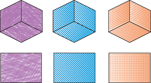
19.6 Patterns and Hatching
Artists and engineers use patterns and hatching for a variety of purposes (see Figure 19.7). In engineering drawings patterns and hatch marks are used to distinguish between different material types. In 2D presentation graphics, monochrome and colored patterns and hatches are used for decorative purposes. In artistic renderings, hatching is used to provide visual cues for surface texture, lighting, tone, and shadows.
The OpenGL pipeline can be used to render patterns and hatches using a number of methods. The glPolygonStipple command provides a simple mechanism to apply a repeating 32×32 pattern to a polygon. The stipple pattern acts as a mask that discards rasterized fragments wherever the stipple pattern is zero and allows them to pass wherever the pattern is one. The pattern is aligned to the x and y window coordinate axes and the origin of the pattern is fixed relative to the origin of the window.
Another way to generate the effect of a stipple pattern is to create a mask in the stencil buffer and apply a stenciling operation to polygons as they are drawn. The pattern can be created in the stencil buffer by writing it as a stencil image using glDrawPixels or by drawing geometry elements that set the contents of the stencil buffer. A polygon can be shaded with hatch lines of arbitrary orientation by initializing the stencil buffer with the polygon and using it as a mask during line drawing. The lines can be drawn so that they cover the 2D screen-space bounding rectangle for the object.
Texture mapping provides a more general mechanism for performing pattern fills. The flexible method of assigning and interpolating texture coordinates eliminates the restrictions on patterns being aligned and oriented in window space. A window-coordinate alignment constraint can still be emulated, however, using eye linear texture coordinate generation and a scale and bias transform on the texture matrix stack.
To perform masking operations using texture mapping, several functions are useful. A luminance texture pattern can be used to modulate the polygon color, or an alpha texture can be used with alpha testing or framebuffer blending to either reject fragments outright or to perform weighted blends. The masking technique generalizes to the familiar texture mapping operation in which polygon colors are substituted with the texture colors.
19.6.1 Cross Hatching and 3D Halftones
In (Saito, 1990), Saito suggests using cross hatching to shade 3D geometry to provide visual cues. Rather than performing 2D hatching using a fixed screen space pattern (e.g., using polygon stipple) an algorithm is suggested for generating hatch lines aligned with parametric axes of the object (for example, a sequence of straight lines traversing the length of a cylinder, or a sequence of rings around a cylinder).
A similar type of shading can be achieved using texture mapping. The parametric coordinates of the object are used as the texture coordinates at each vertex, and a 1D or 2D texture map consisting of a single stripe is used to generate the hatching. This method is similar to the methods for generating contour lines in Section 14.10, except that the isocontours are now lines of constant parametric coordinate. If a 1D texture is used, at minimum two alternating texels are needed. A wrap mode of GL_REPEAT is used to replicate the stripe pattern across the object. If a 2D texture is used, the texture map contains a single stripe. Two parametric coordinates can be cross hatched at the same time using a 2D texture map with stripes in both the s and t directions. To reduce artifacts, the object needs to be tessellated finely enough to provide accurate sampling of the parametric coordinates.
This style of shading can be useful with bilevel output devices. For example, a luminance-hatched image can be thresholded against an unlit version of the same image using a max function. This results in the darker portions of the shaded image being hatched, while the brighter portions remain unchanged (as shown in Figure 19.8). The max function may be available as a separate blending extension or as part of the imaging subset. The parameters in the vertex lighting model can also be used to bias it. Using material reflectances that are greater than 1.0 will brighten the image, while leaving self-occluding surfaces black. Alternatively, posterization operations using color lookup tables can be used to quantize the color values to more limited ranges before thresholding. These ideas are generalized to the notion of a 3D halftone screen in (Haeberli, 1993).
Combining the thresholding scheme with (vertex) lighting allows tone and shadow to be incorporated into the hatching pattern automatically. The technique is easily extended to include other lighting techniques such as light maps. Using multipass methods, the hatched object is rendered first to create the ambient illumination. This is followed by rendering diffuse and specular lighting contributions and adding them to the color buffer contents using blending. This converts to a multitexture algorithm by adding the hatch pattern and lighting contributions during texturing. More elaborate interactions between lighting and hatching can be created using 3D textures. Hatch patterns corresponding to different N![]() L values are stored as different r slices in the texture map, and the cosine term is computed dynamically using a vertex program to pass s and t coordinates unchanged while setting r to the computed cosine term.
L values are stored as different r slices in the texture map, and the cosine term is computed dynamically using a vertex program to pass s and t coordinates unchanged while setting r to the computed cosine term.
If fragment programs are supported, more sophisticated thresholding algorithms can be implemented based on the results of intermediate shading computations, either from vertex or fragment shading. Dependent texture lookup operations allow the shape of the threshold function to be defined in a texture map.
Praun et al. (Praun, 2001; Webb, 2002) describe sophisticated hatching techniques using multitexturing with mipmapping and 3D texturing to vary the tone across the surface of an object. They develop procedures for constructing variable hatching patterns as texture maps called tonal art maps as well as algorithms for parameterizing arbitrary surfaces in such a way that the maps can be applied as overlapping patches onto objects with good results.
19.6.2 Halftoning
Halftoning is a technique for trading spatial resolution for an increased intensity range. Intensity values are determined by the size of the halftone. Traditionally, halftones are generated by thresholding an image against a halftone screen. Graphics devices such as laser printers approximate the variable-width circles used in halftones by using circular raster patterns. Such patterns can be generated using a clustered-dot ordered dither (Foley, 1990). An n × n dither pattern can be represented as a matrix. For dithering operations in which the number of output pixels is greater than the number of input pixels (i.e., each input pixel is converted to a n × n set of output pixels) the input pixel is compared against each element in the dither matrix. For each element in which the input pixel is larger than the dither element, a 1 is output; otherwise, a 0. An example 3 × 3 dither matrix is:
A dithering operation of this type can be implemented using the OpenGL pipeline as follows:
1. Replicate the dither pattern in the framebuffer to generate a threshold image the size of the output image. Use glCopyPixels to perform the replication.
2. Set glPixelZoom(n,n) to replicate each pixel to a n×n block.
3. Move the threshold image into the accumulation buffer with glAcciim(GL_LOAD,1.0).
4. Use glDrawPixels to transfer the expanded source image in the framebuffer.
5. Call glAccum(GL_ACCUM,-1.0).
6. Call glAccum(GL_RETURN,-1.0) to invert and return the result.
7. Set up glPixelMap to map 0 to 0 and everything else to 1.0.
8. Call glReadPixels with the pixel map to retrieve the thresholded image.
Alternatively, the subtractive blend function can be used to do the thresholding instead of the accumulation buffer if the imaging extensions are present.2 If the input image is not a luminance image, it can be converted to luminance using the techniques described in Section 12.3.5 during the transfer to the framebuffer. If the framebuffer is not large enough to hold the output image, the source image can be split into tiles that are processed separately and merged.
19.7 2D Drawing Techniques
While most applications use OpenGL for rendering 3D data, it is inevitable that 3D geometry must be combined with some 2D screen space geometry. OpenGL is designed to coexist with other renderers in the window system, meaning that OpenGL and other renderers can operate on the same window. For example, X Window System 2D drawing primitives and OpenGL commands can be combined together on the same surface. Similarly, Win32 GDI drawing and OpenGL commands can be combined in the same window.
One advantage of using the native window system 2D renderer is that the 2D renderers typically provide more control over 2D operations and a richer set of built-in functions. This extended control may include joins in lines (miter, round, bevel) and end caps (round, butt). The 2D renderers also often specify rasterization rules that are more precise and therefore easier to predict or portably reproduce the results. For example, both the X Window System and Win32 GDI have very precise specifications of the algorithms for rasterizing 2D lines, whereas OpenGL has provided some latitude for implementors that occasionally causes problems with application portability.
Some disadvantages in not using OpenGL commands for 2D renderings are:
• The native window system 2D renderers are not tightly integrated with the OpenGL renderers.
• The 2D renderer cannot query or update additional OpenGL window states such as the depth, stencil, or other ancillary buffers.
• The 2nd coordinate system typically has the origin at the top left corner of the window.
• Some desirable OpenGL functionality may not be available in the 2D renderer (framebuffer blending, antialiased lines).
• The 2D code is less portable; OpenGL is available on many platforms, whereas specific 2D renderers are often limited to particular platforms.
19.7.1 Accuracy in 2D Drawing
To specify object coordinates in window coordinates, an orthographic projection is used. For a window of width w and height h, the transformation maps object coordinate (0, 0) to window coordinate (0, 0) and object coordinate (w, h) to window coordinate (w, h). Since OpenGL has pixel centers on half-integer locations, this mapping results in pixel centers at 0.5, 1.5, 2.5, …, w − .5 along the x axis and 0.5, 1.5, 2.5, …, h − .5 along the y axis.
One difficulty is that the line (and polygon) rasterization rules for OpenGL are designed to avoid multiple writes (hits) to the same pixel when drawing connected line primitives. This avoids errors caused by multiple writes when using blending or stenciling algorithms that need to merge multiple primitives reliably. As a result, a rectangle drawn with a GL_LINE_LOOP will be properly closed with no missing pixels (dropouts), whereas if the same rectangle is drawn with a GL_LINE_STRIP or independent GL_LINES there will likely be pixels missing and/or multiple hits on the rectangle boundary at or near the vertices of the rectangle.
A second issue is that OpenGL uses half-integer pixel centers, whereas the native window system invariably specifies pixel centers at integer boundaries. Application developers often incorrectly use integer pixel centers with OpenGL without compensating in the projection transform. For example, a horizontal line drawn from integer coordinates (px, py) to (qx, py) with px < qx will write to pixels with pixel centers at window x coordinate px + .5, px + 1.5, px + 2.5, …, qx−.5, and not the pixel with center at qx + .5. Instead, the end points of the line should be specified on half-integer locations. Conversely, for exact position of polygonal primitives, the vertices should be placed at integer coordinates, since the behavior of a vertex at a pixel center is dependent on the point sampling rules used for the particular pipeline implementation.
19.7.2 Line Joins
Wide lines in OpenGL are drawn by expanding the width of the line along the x or y direction of the line for y-major and x-major lines, respectively (a line is x-major if the slope is in the range [−1, 1]). When two noncolinear wide lines are connected, the overlap in the end caps leaves a noticeable gap. In 2D drawing engines such as GDI or the X Window System, lines can be joined using a number of different styles: round, mitered, or beveled as shown in Figure 19.9.

A round join can be implemented by drawing a round antialiased point with a size equal to the line width at the shared vertex. For most implementations the antialiasing algorithm generates a point that is similar enough in size to match the line width without noticeable artifacts. However, many implementations do not support large antialiased point sizes, making it necessary to use a triangle fan or texture-mapped quadrilateral to implement a disc of the desired radius to join very wide lines.
A mitered join can be implemented by drawing a triangle fan with the first vertex at the shared vertex of the join, two vertices at the two outside vertices of rectangles enclosing the two lines, and the third at the intersection point created by extending the two outside edges of the wide lines. For an x-major line of width w and window coordinate end points (x0, y0) and (x1, y1) the rectangle around the line is (x0, y0 − (w − 1)/2), (x0, y0 − (w − 1)/2 + w), (x1, y1 − (w − 1)/2 + w), (x1, y1 − (w − 1)/2).
Mitered joins with very sharp angles are not aesthetically pleasing, so for angles less then some threshold angle (typically 11 degrees) a bevel join is used. A bevel join can be constructed by rendering a single triangle consisting of the shared vertex and the two outside corner vertices of the lines as previously described.
Having gone this far, it is a small step to switch from using lines to using triangle strips to draw the lines instead. One advantage of using lines is that many OpenGL implementations support antialiasing up to moderate line widths, whereas there is substantially less support for polygon antialiasing. Wide antialiased lines can be combined with antialiased points to do round joins, but it requires the overlap algorithm from Section 16.7.5 to sort the coverage values. Accumulation buffer antialiasing can be used with triangle primitives as well.
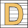
19.7.3 2D Trim Curves
Many 2D page display languages and drawing applications support the creation of shapes with boundaries defined by quadratic and cubic 2D curves. The resulting shapes can then be shaded using a variety of operators. Using many of the shading algorithms previously described, an OpenGL implementation can perform the shading operations; however, the OpenGL pipeline only operates on objects defined by polygons. Using the OpenGL pipeline for shapes defined by higher-order curves might require tessellating the curved shapes into simple polygons, perhaps using the GLU NURBS library. A difficulty with this method is performing consistent shading across the entire shape. To perform correct shading, attributes values such as colors and texture coordinates must be computed at each of the vertices in the tessellated object.
An equivalent, but simpler, method for rendering complex shapes is to consider the shape as a 2D rectangle (or trapezoid) that has parts of the surface trimmed away, using the curved surfaces to define the trim curves. The 2D rectangle is the window-axis-aligned bounding rectangle for the shape. Shading algorithms, such as radial color gradient fills, are applied directly to the rectangle surface and the final image is constructed by masking the rectangle. One method for performing the masking is using the stencil buffer. In this method the application scan converts the trim curve definitions, producing a set of trapezoids that define either the parts of the shape to be kept or the parts to be removed (see Figure 19.10). The sides of the trapezoids follow the curve definitions and the height of each trapezoid is determined by the amount of error permissible in approximating the curve with a straight trapezoidal edge. In the worst case, a trapezoid will be 1 pixel high and can be rendered as a line rather than a polygon. Figure 19.10 exaggerates the size of the bounding rectangle for clarity; normally it would tightly enclose the shape.
Evaluating the trim curves on the host requires nontrivial computation, but that is the only pixel-level host computation required to shade the surface. The trim regions can be drawn efficiently by accumulating the vertices in a vertex array and drawing all of the regions at once. To perform the shading, the stencil buffer is cleared, and the trim region is created in it by drawing the trim trapezoids with color buffer updates disabled. The bounding rectangle is then drawn with shading applied and color buffer updates enabled.
To render antialiased edges, a couple of methods are possible. If multisample antialiasing is supported, the supersampled stencil buffer makes the antialiasing automatic, though the quality will be limited by the number of samples per pixel. Other antialiasing methods are described in Chapter 10. If an alpha buffer is available, it may serve as a useful antialiased stenciling alternative. In this algorithm, all trapezoids are reduced to single-pixel-high trapezoids (spans) and the pixel coverage at the trim curve edge is computed for each span. First, the boundary rectangle is used to initialize the alpha buffer to one with updates of the RGB color chennels disabled. The spans are then drawn with alpha values of zero (color channel updates still disabled). Next, the pixels at the trim curve edges are redrawn with their correct coverage values. Finally, color channel updates are enabled and the bounding rectangle is drawn with the correct shading while blending with source and destination factors of GL_ONE_MINUS_DST_ALPHA and GL_ZERO. The factor GL_ONE_MINUS_DST_ALPHA is correct if the coverage values correspond to the nonvisible part of the edge pixel. If the trim regions defined the visible portion, GL_DST_ALPHA should be used instead.
A simple variation computes the alpha map in an alpha texture map rather than the alpha buffer and then maps the texels to pixel fragments one to one. If color matrix functionality (or fragment programs) is available, the alpha map can be computed in the framebuffer in one of the RGB channels and then swizzled to the alpha texture during a copy-to-texture operation (Section 9.3.1).
By performing some scan conversion within the application, the powerful shading capabilities of the OpenGL pipeline can be leveraged for many traditional 2D applications. This class of algorithms uses OpenGL as a span processing engine and it can be further generalized to compute shading attributes at the start and end of each span for greater flexibility.
19.8 Text Rendering
Text rendering requirements can vary widely between applications. In illustration applications, text can play a minor role as annotations on an engineering drawing or can play a central role as part of a poster or message in a drawing. Support for drawing text in 2D renderers has improved substantially over the past two decades. In 3D renderers such as OpenGL, however, there is little direct support for text as a primitive.
OpenGL does provide ample building blocks for creating text-rendering primitives, however. The methods for drawing text can be divided into two broad categories: image based and geometry based.
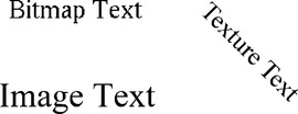
19.8.1 Image-based Text
Image-based primitives use one of the pixel image-drawing primitives to render separate pixel images for each character. The OpenGL glBitmap primitive provides support for traditional single-bit-per-pixel images and resembles text primitives present in 2D renderers. To leverage the capabilities of the host platform, many of the OpenGL embedding layers include facilities to import font data from the 2D renderer, for example, glXUseXFont in the GLX embedding and wglUseFontBitmaps in WGL.
Typically the first character in a text string is positioned in 3D object coordinates using the glRasterPos command, while the subsequent characters are positioned in window (pixel) coordinates using offsets specified with the previously rendered character. One area where the OpenGL bitmap primitive differs from typical 2D renderers is that positioning information is specified with floating-point coordinates and retains subpixel precision when new positions are computed from offsets. By transforming the offsets used for positioning subsequent characters, the application can render text strings at angles other than horizontal, but each character is rendered as a window-axis-aligned image.
The bitmap primitive has associated attributes that specify color, texture coordinates, and depth values. These attributes allow the primitive to participate in hidden surface and stenciling algorithms. The constant value across the entire primitive limits the utility of these attributes, however. For example, color and texture coordinates cannot directly vary across a bitmap image. Nevertheless, the same effect can be achieved by using bitmap images to create stencil patterns. Once a pattern is created in the stencil buffer, shaded or texture-mapped polygons that cover the window extent of the strings are drawn and the fragments are written only in places where stencil bits have been previously set.
Display List Encodings
In the most basic form, to draw a character string an application draws issues a glBitmap command for each character. To improve the performance and simplify this process, the application can use display lists. A contiguous range of display list names are allocated and associated with a corresponding contiguous range of values in the character set encoding. Each display list contains the bitmap image for the corresponding character. List names obey the relationship n = c + b, where c is a particular character encoding, n is the corresponding list name, and b is the list name corresponding to encoding 0. Once the display lists have been created, a string is drawn by setting the list base b (using glListBase) and then issuing a single glCallLists command with the pointer to the array containing the string.
For strings represented using byte-wide array elements, the GL_UNSIGNED_BYTE type is used. This same method is easily adapted to wider character encodings, such as 16-bit Unicode, by using a wider type parameter with the glCallLists command. If the character encoding is sparse, it may be advantageous to allocate display list names only for the nonempty encodings and use an intermediate table to map a character encoding to a display list name. This changes the string-drawing algorithm to a two-step process: first a new array of display list names is constructed from the string using the look-up table, then the resulting array is drawn using glCallLists.
Many applications use multiple graphical representations for the same character encoding. The multiple representations may correspond to different typefaces, different sizes, and so on. Using the direct one-to-one display list mapping, each representation has a different display list base. Using the look-up table mapping, each representation has a separate table.
Kerning
More sophisticated applications may wish to implement kerning to tune the spacing between different character pairs. Since the character advance is dependent on the last rendered character and the current character, a single advance cannot be stored in the same display list with each character. However, a kerning table can be computed containing an adjustment for each pair of characters and each unique adjustment can be encoded in a separate display list. A simple method for making a relative adjustment to the raster position (without drawing any pixels) is to issue a glBitmap command with a zero-size image, specifying the desired adjustment as the offset parameters.
A variation on the two-step text-rendering method can be used to build a kerned string. The array of list names constructed in the first step also includes a call to the display list containing the corresponding adjustment found in the kerning table. The resulting array contains an alternating sequence of lists to draw a character and lists to adjust the position. A single glCallLists command can draw the entire string using the constructed array in the second step. Ligatures and other features can also be accommodated by storing them as separate display lists and incorporating them when building the array of lists.
Pixmap Images
Another limitation with the bitmap primitive is that it cannot be used to render antialiased text. This limitation can be overcome by using the glDrawPixels command to draw character images that have been preantialiased (prefiltered). Antialiased character images store both a luminance (or RGB color) and alpha coverage values and are rendered using the over compositing operator described in Section 11.1.1.
The glDrawPixels primitive doesn’t include offsets to advance the raster position to the next character position, so the application must compute each character position and use the glRasterPos command to move the current raster position. It is probable that the application needs to position the subsequent characters in a string in window coordinates rather than object coordinates.
Another way to implement relative positioning is to define the raster position in terms of a relative coordinate system in which each character is drawn with raster position object coordinates (0, 0, 0). A cumulative character advance is computed by concatenating a translation onto the modeling transform after each character is drawn. The advantage of such a scheme is that display lists can still be used to store the glRasterPos, glDrawPixels, and glTranslatef commands so that a complete string can be drawn with a single invocation of glCallLists. However, at the start and end of the string additional modeling commands are required to establish and tear down the coordinate system.
Establishing the coordinate system requires computing a scaling transform that maps (x, y) object coordinates one-to-one to window coordinates. Since this requires knowledge of the current cumulative modelview and projection transforms, it may be difficult to transparently incorporate into an application. Often applications will save and restore the current modelview and projection transforms rather than track the cumulative transform. Saving the state can have deleterious performance effects, since state queries typically introduce “bubbles” of idle time into the rendering pipeline. An alternative to saving and restoring state is to specify the raster position in window coordinates directly using the ARB_window_pos extension.3 Unfortunately, using absolute positioning requires issuing a specific raster position command for each character position, eliminating the opportunity to use position independent display lists. Establishing a window coordinate system transform and using relative positioning is a more broadly applicable method for working with both the image- and geometry-based rendering techniques.
Texture Images
Using RGB images allows the color to vary within a single character, though the color values need to be assigned to the image data before transfer to the pipeline. A common limitation with both bitmap and pixel image character text rendering is that the text cannot be easily scaled or rotated. Limited scaling can be achieved using pixel zoom operations, but no filtering is performed on the images so the results deteriorate very quickly.
A third type of image-based text stores the character glyphs as texture maps and renders them as quadrilaterals using the billboard techniques described in Section 13.5 (Haeberli, 1993; Kilgard, 1997). Using billboard geometry allows text strings to be easily rotated and texture filtering allows scaling over a larger range than pixel zoom. Using mipmap filtering increases the effective scaling range even more. In addition to affine scaling, the text strings can be perspective projected since the characters are affixed to regular geometry. Text can be shaded with a color gradient or lit by lighting and shading the underlying quad and modulating it with the texture map. If the source image for the texture map is antialiased, the rendered text remains antialiased (within the limitations of the texture filter).
The images used in the texture maps are the same images that are used for pixmap text rendering. The texture maps are constructed directly from the pixel image sources and are also rendered using compositing techniques. The characters stored in the texture maps can also be rendered with other geometry besides simple screen parallel quads. They can be decaled directly onto other geometry, combined with stencil operations to create cutouts in the geometry, or projected onto geometry using the projection techniques described in Section 14.9.
The high performance of texture mapping on modern hardware accelerators makes rendering using texture-mapped text very fast. To maximize the rendering efficiency it is desirable to use the mosaicing technique described in Section 14.4 to pack the individual font glyphs into a single texture image. This avoids unnecessarily padding individual character glyphs to a power-of-two image. Individual glyphs are efficiently selected by setting the texture coordinates to index the appropriate subimage rather than binding a new texture for each character. All character positioning is performed in object space. To position subsequent characters in the string using window coordinates, variations on the method described for moving the raster position can be used.
19.8.2 Geometry-based Text
Geometry-based text is rendered using geometric primitives such as lines and polygons.4 Text rendered using 3D primitives has several advantages: attributes can be interpolated across the primitive; character shapes have depth in addition to width and height; character geometry can be easily scaled, rotated, and projected; and the geometry can be antialiased using regular antialiasing techniques.
Characters rendered using a series of arc and line segment primitives are called stroke or vector fonts. They were originally used on vector-based devices such as calligraphic displays and pen plotters. Stroke fonts still have some utility in raster graphics systems since they are efficient to draw and can be easily rotated and scaled. Stroke fonts continue to be useful for complex, large fonts such as those used for Asian languages, since the storage costs can be significantly lower than other image- or geometry-based representations. They are seldom used for high-quality display applications since they suffer from legibility problems at low resolutions and at larger scales the stroke length appears disproportionate relative to the line width of the stroke. This latter problem is often alleviated by using double or triple stroke fonts, achieving a better sense of width by drawing parallel strokes with a small separation between them (Figure 19.12).

The arc segments for stroke fonts are usually tessellated to line segments for rendering. Ideally this tessellation matches the display resolution, but frequently a one-time tessellation is performed and only the tessellated representation is retained. This results in blocky rather than smooth curved boundaries at higher display resolutions. Rendering stroke fonts using the OpenGL pipeline requires little more than rendering line primitives. To maximize efficiency, connected line primitives should be used whenever possible. The line width can be varied to improve the appearance of the glyphs as they are scaled larger and antialiasing is implemented using regular line antialiasing methods (Section 10.4).
Applications can make more creative use of stroke fonts by rendering strokes using primitives other than lines (such as using flat polygons or 3D cylinders and spheres). Flat polygons traced along each stroke emulate calligraphic writing, while 3D solid geometry is created by treating each stroke as a path and a profile is swept along the path. Tools for creating geometry from path descriptions are common in most modeling packages.
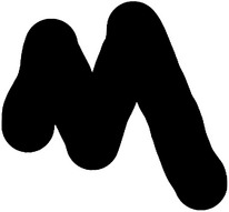
Outline Fonts
Outline font is the term used for the resolution-independent mathematical description of a font. Type 1 and TrueType are examples of systems for describing fonts as series of 2D closed curves (contours). Outline fonts are converted to bitmaps by scaling the outline to a particular size and then scan-converting the contours, much like scan-converting a polygon. Alternatively, the contours can be tessellated into polygonal geometry or a set of line segments for rendering as filled polygons or outlines. The curves can also be used to generate profiles for generating 3D extrusions, converting them to a mesh of polygons. Since the process starts with a resolution independent representation, outline fonts can produce high-quality polygonal or vector representations at almost any resolution. It is “almost” any resolution, since low resolutions usually require some additional hinting beyond the curve descriptions to improve the legibility.

To render outline fonts using OpenGL, an application requires a font engine or library to convert the mathematical contour description into polygons or lines. Some platform embeddings include such a feature directly; for example, the Microsoft WGL embedding includes wglUseFontOutlines, to generate display lists of polygon or line representations from TrueType font descriptions. On other systems, readily available font libraries, such as the FreeType project (FreeType, 2003), can be used to generate pixmap images directly, and to retrieve contour descriptions. The curves comprising the contours are converted to vectors by evaluating the curve equations and creating line segments that approximate the curves within a specified tolerance. The vector contours are then drawn as outlines or tessellated to polygons using the GLU tessellator. Simple extrusions can be generated from the resulting tessellation, using the meshes for the front and back faces of each character and using the vector contours to generate the side polygons bridging the faces.
19.9 Drawing and Painting
Content creation applications often provide the digital equivalent of traditional drawing and painting techniques, in which the user adds color to pixel values using pens and brushes with a variety of shapes and other properties. There are many advantages that come from performing the operations digitally: the ability to undo operations; the ability to automate repetitive tasks, the availability of a unified palette of different painting techniques, and (to some extent) the ability to operate independent of the output resolution. There are many commercial drawing and painting packages that provide these features. Many of them can take advantage of the facilities available in the OpenGL 3D pipeline to accelerate operations. These techniques go beyond the idea of simply using the 3D pipeline to incorporate 3D geometry into an image.
Smooth shading provides a simple way to perform color gradient fills, while 1D and 2D texture mapping allow more flexible control over the shape of the gradients. Texture mapping provides additional opportunities for implementing irregularly shaped brush geometry by combining customized geometry and texture alpha to define the brush shape (see Figure 19.14). A brush stroke is rendered by sampling the coordinates of an input stroke, rendering the brush geometry centered about each input sample. Typically the input coordinate samples are spaced evenly in time, allowing dense strokes to be created by moving the input device slowly and light strokes by moving it quickly. Alternatively, a pressure-sensitive input device can be used, mapping input pressure to density.
Using texture-mapped brush geometry allows two types of painting algorithms to be supported. In the first style, the texture-mapped brush creates colored pixel fragments that are blended with the image in the color buffer in much the same way a painter applies paint to a painting. The second method uses the brush geometry and resulting brush strokes to create a mask image, Im, used to composite a reference image, Ir, over the original image, Io, using the strokes to reveal parts of the reference image:
The reference image is often a version of the original image created using a separate processing or filtering algorithm (such as, a blurring or sharpening filter). In this way, brush strokes are used to specify the parts of the original image to which the filtering algorithm is applied without needing to compute the filter dynamically on each stroke.
There are several ways to implement the revealing algorithm. If an alpha buffer is available, the brush strokes can incrementally add to an alpha mask in the alpha buffer. An alpha buffer allows rendering of antialiased or smooth stroke edges. If an alpha buffer isn’t available, the stencil buffer can be used instead. The alpha or stencil buffer is updated as the strokes are drawn and an updated image is created each frame by compositing a buffer storing the reference image with a buffer storing the original image. The compositing operation is performed using either blending or stencil operations with a buffer-to-buffer pixel copy.
If the application is using double buffering, either aux buffers or off-screen buffers can be used to hold the original and reference image, recopying the original to the back buffer each frame, before compositing the reference image on top. Both images can also be stored as texture maps and be transferred to the framebuffer by drawing rectangles that project the texels one-to-one to pixels. Other variations use multitexture to composite the images as part of rendering texture rectangles. Brush strokes are accumulated in one of the RGB channels of an off-screen color buffer and copied to an alpha texture map using color matrix swizzling (Section 9.3.1) before rendering each frame.
19.9.1 Undo and Resolution Independence
One of the advantages of performing painting operations digitally is that they can be undone. This is accomplished by recording all of the operations that were executed to produce the current image (sometimes called an adjustment layer). Each brush stroke coordinate is recorded as well as all of the parameters associated with the operation performed by the brush stroke (both paint and reveal). This allows every intermediate version of the image to be reconstructed by replaying the appropriate set of operations. To undo an operation, the recorded brush strokes are deleted. Interactive performance can be maintained by caching one of the later intermediate images and only replaying the subsequent brush strokes. For example, for the revealing algorithm, when a new reference image is created to reveal, a copy of the current image is saved as the original image; only the set of strokes accumulated as part of revealing this reference image is replayed each frame.
Erase strokes are different from undo operations. Erase strokes have the effect of selectively undoing or erasing part of a brush stroke. However, undo operations also apply to erase strokes. Erase strokes simply perform local masking operations to the current set of brush strokes, creating a mask that is applied against the stroke mask. Erase strokes are journaled and replayed in a manner similar to regular brush strokes.
Since all of the stroke geometry is stored along with the parameters for the filtering algorithms used to create references images for reveals, it is possible to replay the brush strokes using images of different sizes, scaling the brush strokes appropriately. This provides a degree of resolution independence, though in some cases changing the size of the brush stroke may not create the desired effect.
19.9.2 Painting in 3D
A texture map can be created by “painting” an image, then viewing it textured on a 3D object. This process can involve a lot of trial and error. Hanrahan (1990) and Haeberli proposed methods for creating texture maps by painting directly on the 2D projection of the 3D geometry (see Figure 19.15). The two key problems are determining how screen space brush strokes are mapped to the 3D object coordinates and how to efficiently perform the inverse mapping from geometry coordinates to texture coordinates.
In the Hanrahan and Haeberli method an object into a quadrilateral mesh, making the number of quadrilaterals equal to the size of the texture map. This creates an approximate one-to-one correspondence between texels in the texture map and object geometry. The object tagging selection technique (described in Section 16.1.2) is used to efficiently determine which quads are covered by a brush stroke. Once the quads have been located, the texels are immediately available. Brush geometry can be projected onto the object geometry using three different methods: object parametric, object tangent plane, or screen space.
Object parametric projection maps brush geometry and strokes to the s and t texture coordinate parameterization of the vector. As the brush moves the brush geometry is decaled to the object surface. Object tangent projection considers the brush geometry as an image, tangent to the object surface (perpendicular to the surface normal) at the brush center and projects the brush image onto the object. As the brush moves, the brush image remains tangent to the object surface. The screen space projection keeps the brush aligned with the screen (image plane). In the original Hanrahan and Haeberli algorithm, the tangent and screen space brushes are implemented by warping the images into the equivalent parametric projection. The warp is computed within the application and used to update the texture map.
The preceding scheme uses a brute-force geometry tessellation to implement the selection algorithm. An alternative method that works well with modern graphics accelerators with high performance (and predictable) texture mapping avoids the tessellation step and operates directly on a 2D texture map. The object identifiers for the item buffer are stored in one 2D texture map, called the tag texture and a second 2D texture map stores the current painted image, called the paint texture. To determine the location of the brush within the texture image, the image is drawn using the tag texture with nearest filtering and a replace environment function. This allows the texture coordinates to be determined directly from the color buffer. The paint texture can be created in the framebuffer. For object parametric projections, the current brush is mapped and projected to screen space (parameter space) as for regular 2D painting. For tangent and screen space projections, the brush image is warped by tessellating the brush and warping the vertex coordinates of the brush. As changes are made to the paint texture, it is copied to texture memory and applied to the object to provide interactive feedback.
To compute the tangent space projection, the object’s surface normal corresponding to the (s, t) coordinates is required. This can be computed by interpolating the vertex normals of the polygon face containing the texture coordinates. Alternatively, a second object drawing pass can draw normal vectors as colors to the RGB components of the color buffer. This is done using normal map texture coordinate generation combined with a cube map texture containing normal vectors. The normal vector can be read back at the same brush location in the color buffer as for the (s, t) coordinates. Since a single normal vector is required, only one polygon containing the texture coordinate need be drawn.
The interactive painting technique can be used for more than applying color to a texture map. It can be used to create light intensity or more general material reflectance maps for use in rendering the lighting effects described in Chapter 15. Painting techniques can also be used to design bump or relief maps for the bump map shading techniques described in Section 15.10 or to interactively paint on any texture that is applied as part of a shading operation.
19.9.3 Painting on Images
The technique of selectively revealing an underlying image gives rise to a number of painting techniques that operate on images imported from other sources (such as digital photographs). One class of operations allows retouching the image using stroking operations or other input methods to define regions on which various operators are applied. These operators can include the image processing operations described in Chapter 12: sharpen, blur, contrast enhancement, color balance adjustment, and so on.
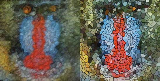
Haeberli (1990) describes a technique for using filters in the form of brush strokes to create abstract images (impressionistic paintings) from source images. The output image is generated by rendering an ordered list of brush strokes. Each brush stroke contains color, shape, size, and orientation information. Typically the color information is determined by sampling the corresponding location in the source image. The size, shape, and orientation information are generated from user input in an interactive painting application. The paper also describes some novel algorithms for generating brush stroke geometry. One example is the use of a depth buffered cone with the base of the cone parallel to the image plane at each stroke location. This algorithm results in a series of Dirichlet domains (Preparata, 1985) where the color of each domain is sampled from the source image (see Figure 19.16).
Additional effects can be achieved by preprocessing the input image. For example, the contrast can be enhanced, or the image sharpened using simple image-processing techniques. Edge detection operators can be used to recover paths for brush strokes to follow. These operations can be automated and combined with stochastic methods to choose brush shape and size to generate brush strokes automatically.
19.10 Summary
Illustration and artistic techniques is a broad area of active research. This chapter sampled some algorithms and ideas from a few different areas, but we have just scratched the surface. There are several excellent books that cover the topic of nonphotorealistic rendering in greater detail. The addition of the programmable pipeline will undoubtedly increase the opportunities for innovation on both the artistic side and the pursuit of higher-quality rendered images.