13.1 Computing Inverse Transforms Efficiently

In general, when geometry is transformed by a 4×4 matrix, normals or other vectors associated with that geometry have to be transformed by the inverse transpose of that matrix. This is done to preserve angles between vectors and geometry (see Section 2.3 for details). Finding the inverse transpose of a general 4× 4 matrix can be an expensive computation, since it requires inverting a full 4×4 matrix. The general procedure is shown below; a matrix M is inverted to M′, then transposed.

OpenGL performs this computation for the application as part of the transform pipeline, which provides the functionality needed for basic lighting, texture coordinate generation, and environment operations. There are times when an application may need to construct more complex transforms not provided in the pipeline. Some techniques require a special per-vertex vector, such as the bi-normal vector used in bump mapping (Section 15.10) and anisotropic lighting (Section 15.9.3). Other algorithms, such as those modeling curved reflectors (Section 17.1.3) subdivide surfaces based on the values of adjacent normal or reflection vectors. In these, and many other algorithms, an efficient way to compute vector transform matrices is needed.

Although finding the inverse of a general 4×4 matrix is expensive, many graphics applications use only a small set of matrix types in the modelview matrix, most of which are relatively easy to invert. A common approach, used in some OpenGL implementations, is to recognize the matrix type used in the modelview matrix (or tailor the application to limit the modelview matrix to a given type), and apply an appropriate shortcut. Matrix types can be identified by tracking the OpenGL commands used to create them. This can be simple if glTranslate, glScale, and glRotate commands are used. If glLoadMatrix or glMultMatrix are used, it’s still possible to rapidly check the loaded matrix to see if it matches one of the common types. Once the type is found, the corresponding inverse can be applied. Some of the more common matrix types and inverse transpose shortcuts are described below.

An easy (and common) case arises when the transform matrix is composed of only translates and rotates. A vector transformed by the inverse transpose of this type of matrix is the same as the vector transformed by the original matrix, so no inverse transpose operation is needed.

If uniform scale operations (a matrix M with elements m₁₁ = m₂₂ = m₃₃ = s) are also used in the transform, the length of the transformed vector changes. If the vector length doesn’t matter, no inverse is needed. Otherwise, renormalization or rescaling is required. Renormalization scales each vector to unit length. While renormalization is computationally expensive, it may be required as part of the algorithm anyway (for example, if unit normals are required and the input normals are not guaranteed to be unit length). Rescaling applies an inverse scaling operation after the transform to undo its scaling effect. Although it is less expensive than renormalization, it won’t produce unit vectors unless the untransformed vectors were already unit length. Rescaling uses the inverse of the transform’s scaling factor, creating a new matrix ; the diagonal element’s scale factor is inverted and used to scale the matrix.

Table 13.1 summarizes common shortcuts. However, it’s not always practical to characterize the matrix and look up its corresponding inverse shortcut. If the modelview transform is constructed of more than translates, rotates, and uniform scales, computing the inverse transpose is necessary to obtain correct results. But it’s not always necessary to find the full inverse transpose of the composited transform.

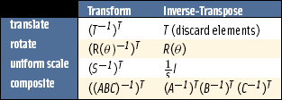
An inverse transpose of a composite matrix can be built incrementally. The elements of the original transform are inverted and transposed individually. The resulting matrices can then be composed, in their original order, to construct the inverse transpose of the original sequence. In other words, given a composite matrix built from matrices A, B, and C, ((ABC)⁻¹)^T is equal to (A⁻¹)^T(B⁻¹)^T(C⁻¹)^T. Since these matrices are transposed, the order of operations doesn’t change. Many basic transforms, such as pure translates, rotates, and scales, have trivial special case inversions, as shown previously. The effort of taking the inverse transpose individually, then multiplying, can be much less in these cases.

If the transform is built from more complex pieces, such as arbitrary 4×4 matrices, then using an efficient matrix inversion algorithm may become necessary. Even in this case, trimming down the matrix to 3×3 (all that is needed for transforming vectors) will help.

13.2 Stereo Viewing

Stereo viewing is used to enhance user immersion in a 3D scene. Two views of the scene are created, one for the left eye, one for the right. To display stereo images, a special display configuration is used, so the viewer’s eyes see different images. Objects in the scene appear to be at a specific distance from the viewer based on differences in their positions in the left and right eye views. When done properly, the positions of objects in the scene appear more realistic, and the image takes on a solid feeling of “space”.

OpenGL natively supports stereo viewing by providing left and right versions of the front and back buffers. In normal, non-stereo viewing, the default buffer is the left one for both front and back. When animating stereo, both the left and right back buffers are used, and both must be updated each frame. Since OpenGL is window system independent, there are no interfaces in OpenGL for stereo glasses or other stereo viewing devices. This functionality is part of the OpenGL/Window system interface library; the extent and details of this support are implementation-dependent and varies widely.

A stereo view requires a detailed understanding of viewer/scene relationship (Figure 13.1). In the real world, a viewer sees two separate views of the scene, one for each eye. The computer graphics approach is to create a transform to represent each eye’s view, and change other parameters for each view as needed by the stereo display hardware. Since a real viewer will shift view direction to focus on an object of interest, an OpenGL application does the same. Ideally, the eye transforms are updated based on the object the user of the stereo application is looking at, but this requires some method of tracking the viewer’s focus of attention.

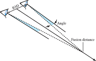
A less ambitious technique uses the viewing direction instead, and stereo parameters that describe the position of the left and right eyes. The model requires that both eye views are aimed at a single point along the line of sight; another stereo parameter is added to represent the distance to that point from the eye point. This parameter is called the fusion distance (FD). When the two scenes are rendered together to form a stereo image, objects at this distance will appear to be embedded in the front surface of the display (“in the glass”). Objects farther than the fusion distance from the viewer will appear to be “behind the glass” while objects in front will appear to float in front of the display. The latter effect can be hard to maintain, since objects visible to the viewer beyond the edge of the display tend to destroy the illusion.

To compute the left and right eye views, the scene is rendered twice, each with the proper eye transform. These transforms are calculated so that the camera position, view, direction and up direction correspond to the view from each of the viewer’s two eyes. The normal viewer parameters are augmented by additional information describing the position of the viewer’s eyes, usually relative to the traditional OpenGL eye point. The distance separating the two eyes is called the interocular distance or IOD. The IOD is chosen to give the proper spacing of the viewer’s eyes relative to the scene being viewed.

The IOD value establishes the size of the imaginary viewer relative to the objects in the scene. This distance should be correlated with the degree of perspective distortion present in the scene in order to produce a realistic effect.

To formalize the position and direction of views, consider the relationship between the view direction, the view up vector, and the vector separating the two eye views. Assume that the view direction vector, the eye position vector (a line connecting both eye positions), and the up vectors are all perpendicular to each other. The fusion distance is measured along the view direction. The position of the viewer can be defined to be at one of the eye points, or halfway between them. The latter is used in this description. In either case, the left and right eye locations can be defined relative to it.

Using the canonical OpenGL view position, the viewer position is at the origin in eye space. The fusion distance is measured along the negative z-axis (as are the near and far clipping planes). Assuming the viewer position is halfway between the eye positions, and the up vector is parallel to the positive y-axis, the two viewpoints are on either side of the origin along the x-axis at (−IOD/2, 0, 0) and (IOD/2, 0, 0).

Given the spatial relationships defined here, the transformations needed for correct stereo viewing involve simple translations and off-axis projections (Deering, 1992). The stereo viewing transforms are the last ones applied to the normal viewing transforms. The goal is to alter the transforms so as to shift the viewpoint from the normal viewer position to each eye. A simple translation isn’t adequate, however. The transform must also aim each to point at the spot defined by view vector and the fusion distance.

The stereo eye transformations can be created using the gluLookAt command for each eye view. The gluLookAt command takes three sets of three-component parameters; an eye position, a center of attention, and an up vector. For each eye view, the gluLookAt function receives the eye position for the current eye (±IOD/2, 0, 0), an up vector (typically 0, 1, 0), and the center of attention position (0, 0, FD). The center of attention position should be the same for both eye views. gluLookAt creates a composite transform that rotates the scene to orient the vector between the eye position and center of view parallel to the z-axis, then translates the eye position to the origin.

This method is slightly inaccurate, since the rotation/translation combination moves the fusion distance away from the viewer slightly. A shear/translation combination is more correct, since it takes into account differences between a physical stereo view and the properties of a perspective transform. The shear orients the vector between the eye and the center of attention to be parallel to the z-axis. The shear should subtract from x values when the x coordinate of the eye is negative, and add to the x values when the x component of the eye is positive. More precisely, it needs to shear when z equals the −FD. The equation is . Converting this into a 4×4 matrix becomes:

Compositing a transform to move the eye to the origin completes the transform. Note that this is only one way to compute stereo transforms; there are other popular approaches in the literature.

13.3 Depth of Field

The optical equivalent to the standard viewing transforms is a perfect pinhole camera: everything visible is in focus, regardless of how close or how far the objects are from the viewer. To increase realism, a scene can be rendered to vary focus as a function of viewer distance, more accurately simulating a camera with a fixed focal length. There is a single distance from the eye where objects are in perfect focus. Objects farther and nearer to the viewer become increasingly fuzzy.

The depth-of-field problem can be seen as an extension of stereo viewing. In both cases, there are multiple viewpoints, with all views converging at a fixed distance from the viewer on the direction of view vector. Instead of two eye views, the depth of field technique creates a large number of viewpoints that are scattered in a plane perpendicular to the view direction. The images generated from each view rendered are then blended together.

Rendering from these viewpoints generates images which show objects in front of and behind the fusion distance shifted from their normal positions. These shifts vary depending on how far the viewpoint is shifted from the eye position. Like the eye views in stereo viewing, all viewpoints are oriented so their view directions are aimed at a single point located on the original direction of view. As a result, the farther an object is from this aim point, the more the object is shifted from its original position.

Blending these images together combines each set of shifted objects, creating a single blurry one. The closer an object is to the aim point (focal) distance, the less it shifts, and the sharper it appears. The field of view can be expanded by reducing the average amount of viewpoint shift for a given fusion distance. If viewpoints are closer to the original eye point, objects have to be farther from the fusion distance in order to be shifted significantly.

Choosing a set of viewpoints and blending them together can be seen as modeling a physical lens—blending together pinhole views sampled over the lens’ area. Real lenses have a non-zero area, which causes only objects within a limited range of distances to be in perfect focus. Objects closer or farther from the camera focal length are progressively more blurred.

To create depth of field blurring, both the perspective and modelview transforms are changed together to create an offset eye point. A shearing transform applied along the direction of view (-z-axis) is combined into the perspective transform, while a translate is added to the modelview. A shear is chosen so that the changes to the transformed objects are strictly a function of distance from the viewer (the blurriness shouldn’t change based on the perpendicular distance from the view direction), and to ensure that distance of the objects from the viewer doesn’t change.

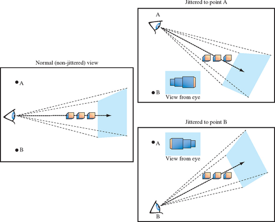
These transform changes can be implemented easily using glfrustum to change the perspective transform, and glTranslate to change the modelview matrix. Given jitter variables xoff and yoff, and a focal length focus, the parameters for the commands are given in Table 13.2.

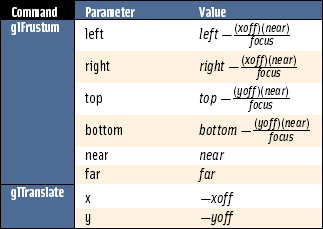
The jitter translation should be the last transform applied in the current modelview sequence, so glTranslate should be called first in the modelview transform code. The final issue to consider is the the number of jitter positions to use, and how to choose those positions. These choices are similar to many other jittering problems. A pattern of irregular positions causes sampling artifacts to show up as noise, rather than more noticeable image patterns. The jitter values shown in Section 10.1 provide good results.

The number of jittered images will be limited to the color resolution available for blending. See Section 11.4.1 for a discussion of blending artifacts and how to calculate blend error. A deep color buffer or accumulation buffer allows more images to be blended together while minimizing blending errors. If the color resolution allows it, and there is time available in the frame to render more images, more samples results in smootherblurring of out of focus objects. Extra samples may be necessary if there are objects close to the viewer and far from the fusion point. Very blurry large objects require more samples in order to hide the fact that they are made of multiple objects.

13.4 Image Tiling

When rendering a scene in OpenGL, the maximum resolution of the image is normally limited to the workstation screen size. For interactive applications screen resolution is usually sufficient, but there may be times when a higher resolution image is needed. Examples include color printing applications and computer graphics images being recorded to film. In these cases, higher resolution images can be divided into tiles that fit within the framebuffer. The image is rendered tile by tile, with the results saved into off-screen memory or written to a file. The image can then be sent to a printer or film recorder, or undergo further processing, such as using down-sampling to produce an antialiased image.

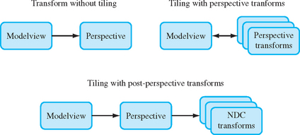
Rendering a large image tile by tile requires repositioning the image to make different tiles visible in the framebuffer. A straightforward way to do this is to manipulate the parameters to glFrustum. The scene can be rendered repeatedly, one tile at a time, by changing the left, right, bottom, and top parameters of glFrustum for each tile.

Computing the argument values is straightforward. Divide the original width and height range by the number of tiles horizontally and vertically, and use those values to parametrically find the left, right, top, and bottom values for each tile.

In these equations each value of i and j corresponds to a tile in the scene. If the original scene is divided into nTiles_horiz by nTiles_vert tiles, then iterating through the combinations of i and j generate the left, right, top, and bottom values for glFrustum to create the tile. Since glFrustum has a shearing component in the matrix, the tiles stitch together seamlessly to form the scene, avoiding artifacts that result from changing the viewpoint. This technique must be modified if gluPerspective or glOrtho is used instead of glFrustum.

There is a better approach than changing the perspective transform, however. Instead of modifying the transform command directly, apply tiling transforms after the perspective one. A subregion of normalized device coordinate (NDC) space corresponding to the tile of interest can be translated and scaled to fill the entire NDC cube. Working in NDC space instead of eye space makes finding the tiling transforms easier, and is independent of the type of projection transform. Figure 13.3 summarizes the two approaches.

For the transform operations to take place after the projection transform, the OpenGL commands must happen before it. A typical sequence of operations is:

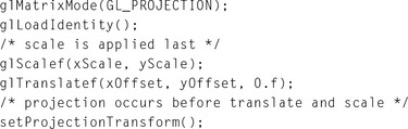
The scale factors xScale and yScale scale the tile of interest to fill the the entire scene:

The offsets xOffset and yOffset are used to offset the tile so it is centered about the z-axis. In this example, the tiles are specified by their lower left corner relative to their position in the scene, but the translation needs to move the center of the tile into the origin of the x-y plane in NDC space:

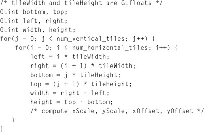
Like the previous example, nTiles_horiz is the number of tiles that span the scene horizontally, while nTiles_vert is the number of tiles that span the scene vertically. Some care should be taken when computing left, bottom, tileWidth, and tileHeight values. It is important that each tile is abutted properly with its neighbors. This can be ensured by guarding against round-off errors. The following code shows an example of this approach. Note that parameter values are computed so that left+tileWidth is guaranteed to be equal to right and equal to left of the next tile over, even if tileWidth has a fractional component. If the frustum technique is used, similar precautions should be taken with the left, right, bottom, and top parameters to glFrustum.

It is worth noting that primitives with sizes that are specified in object space dimensions automatically scale in size. If the scene contains primitives with sizes that are implicitly defined in window space dimensions, such as point sizes, line widths, bitmap sizes and pixel-rectangle, dimensions remain the same in the tiled image. An application must do extra work to scale the window space dimensions for these primitives when tiling.

13.5 Billboarding Geometry

A common shortcut used to reduce the amount of geometry needed to render a scene is to billboard the objects in the scene that have one or more axes of symmetry. Billboarding is the technique of orienting a representation of a symmetrical object toward the viewer. The geometry can be simplified to approximate a single view of an object, with that view always facing the viewer.

This technique works if the object being billboarded has an appearance that doesn’t change significantly around its axis of symmetry. It is also helpful if the objects being billboarded are not a central item in the scene. The principle underlying billboarding is that complexity of an object representation is reduced in a way that is not noticeable. If successful, this approach can reduce the rendering time while maintaining image quality. Good examples of billboarded objects are trees, which have cylindrical symmetry, and clouds which have spherical symmetry. Billboarding can also be a useful technique on its own. For example, text used to annotate objects in a 3D scene can be billboarded to ensure that the text always faces the viewer and is legible.

While simplifying the geometry of an object being billboarded, it is desirable to retain its (possibly complex) outline in order to maintain a realistic result. One way to do this is to start with simple geometry such as a quadrilateral, then apply a texture containing colors that capture the surface detail and alpha components that match the object’s outline. If the texture is rendered with alpha testing or alpha blending enabled, the pattern of alpha values in the texture can control which parts of the underlying geometry are rendered. The alpha texture acts as a per-pixel template, making it possible to cut out complex outlines from simple geometry. For additional details regarding using alpha to trim outlines see Section 11.9.2.

The billboarding technique is not limited to simple texture-mapped geometry though. Billboarding can also be used to draw a tessellated hemisphere, giving the illusion that a full sphere is being drawn. A similar result can be accomplished using backface culling to eliminate rasterization of the back of the sphere, but the vertices for the entire sphere are processed first. Using billboarding, only half of the sphere is transformed and rendered; however, the correct orienting transform must be computed for each hemisphere.

The billboard algorithm uses the object’s modeling transform (modelview transform) to position the geometry, but uses a second transform to hold the object’s orientation fixed with respect to the viewer. The geometry is always face-on to the viewer, presenting a complex image and outline with its surface texture. Typically, the billboard transform consists of a rotation concatenated to the object’s modelview transform, reorienting it. Using a tree billboard as an example, an object with roughly cylindrical symmetry, an axial rotation is used to rotate the simple geometry supporting the tree texture, usually a quadrilateral, about the vertical axis running parallel to the tree trunk.

Assume that the billboard geometry is modeled so that it is already oriented properly with respect to the view direction. The goal is to find a matrix R that will rotate the geometry back into its original orientation after it is placed in the scene by the modelview transform M. This can be done in two steps. Start with the eye vector, representing the direction of view, and apply the inverse of M to it. This will transform the viewing direction vector into object space. Next, find the angle the transformed vector makes relative to canonical view direction in eye space (usually the negative z-axis) and construct a transform that will rotate the angle back to zero, putting the transformed vector into alignment with the view vector.

If the viewer is looking down the negative z-axis with an up vector aligned with the positive y-axis, the view vector is the negative z-axis. The angle of rotation can be determined by computing the vector after being transformed by the modelview matrix M

Applying the correction rotation means finding the angle θ needed to rotate the transformed vector (and the corresponding geometry) into alignment with the direction of view. This can be done by finding the dot product between the transformed vector and the two major axes perpendicular to the axis of rotation; in this case the x and z axes.

where

The sine and cosine values are used to construct a rotation matrix R representing this rotation about the y-axis (V_up). Concatenate this rotation matrix with the modelview matrix to make a combined matrix MR. This combined matrix is the transform applied to the billboard geometry.

To handle the more general case of an arbitrary billboard rotation axis, compute an intermediate alignment rotation A to rotate the billboard axis into the V_up vector. This algorithm uses the OpenGL glRotate command to apply a rotation about an arbitrary axis as well as an angle. This transform rotates the billboard axis into the vertical axis in eye space. The rotated geometry can then be rotated again about the vertical axis to face the viewer. With this additional rotation,

the complete matrix transformation is MAR. Note that these calculations assume that the projection matrix contains no rotational component.

Billboarding is not limited to objects that are cylindrically symmetric. It is also useful to billboard spherically symmetric objects such as smoke, clouds, and bushes. Spherical symmetry requires a billboard to rotate around two axes (up/down and left/right), whereas cylindrical behavior only requires rotation around a single axis (usually up/down) (Figure 13.4). Although it is more general, spherically symmetric billboarding is not suited for all objects; trees, for example, should not bend backward to face a viewer whose altitude increases.

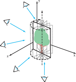
Spherically symmetric objects are rotated about a point to face the viewer. This adds another degree of freedom to the rotation computation. Adding an additional alignment constraint can resolve this degree of freedom, such as one that keeps the object oriented consistently (e.g., constraining the object to remain upright).

This type of constraint helps maintain scene realism. Constraining the billboard to maintain its orientation in object space ensures that the orientation of a plume of smoke doesn’t change relative to the other objects in a scene from frame to frame. A constraint can also be enforced in eye coordinates. An eye coordinate constraint can maintain alignment of an object relative to the screen (e.g., keeping text annotations aligned horizontally).

The computations for a spherically symmetric billboard are a minor extension of those used for the arbitrarily aligned cylindrical one (Figure 13.5). There is still a billboard axis, as there was in the cylindrical case, but now that axis is rotated to vertical alignment before it is used as an axis for the second rotation. An alignment transformation, A, rotates about a vector perpendicular to the billboard’s transformed alignment axis and the up direction. The up direction is either transformed by the modelview matrix, or left untransformed, depending on whether eye-space or object-space alignment is required.

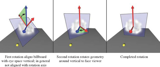
Usually the billboard axis is modeled to be parallel with a major axis in the untransformed geometry. If this is the case, A’s axis of rotation is computed by taking the cross product of the billboard axis and the up vector. In the more general case, if the billboard axis is arbitrary, the transformed billboard axis must be processed before use in the cross product. Project the billboard axis to remove any component parallel to the transformed eye vector, as shown in the following equation.

The sine and cosine of the angle of rotation are computed like they were in the cylindrical case. Cosine is derived from the dot product; sine from the length of the cross product.

A is computed as:

where V_alignment is the billboard alignment axis with the component in the direction of the eye direction vector removed:

Rotation by the A matrix doesn’t change the calculations needed to rotate about the now vertical axis. This means the left/right rotation about the up vector can still be computed from the original modelview transform in exactly the same way as a basic cylindrical billboard.

To compute the A and R matrices, it is necessary to use elements of the geometry’s modelview transform. Retrieving transformation matrices using glGet introduces a large performance penalty on most OpenGL implementations and should be avoided. The application should either read the transformation once per frame, or shadow the current modelview transform to avoid reading it back from OpenGL altogether. Fortunately, it is fairly simple to duplicate the standard OpenGL transform commands in software and provide some simple vector and matrix operations. Matrix equivalents for glTranslate, glRotate, and glScale operations are described in Appendix B. Computing the inverse for each of these three operations is trivial; see Section 13.1 for details.

13.6 Texture Coordinate vs. Geometric Transformations

The texture coordinate pipeline has a significant amount of transformation power. There is a single transformation matrix (called the texture transformation matrix), but it is a full 4×4 matrix with perspective divide functionality. Even if the target is a 2D texture, the perspective divide capability makes the fourth texture coordinate, q, a useful tool, while a 3D texture target can make use of all four coordinates. The texture transform pipeline has nearly the same transformation capabilities as the geometry pipeline, only lacking the convenience of two independent transform matrices and an independent viewport transform.

The texture coordinate path has an additional benefit, automatic texture coordinate generation, which allows an application to establish a linear mapping between vertex coordinates in object or eye space and texture coordinates. The environment mapping functionality is even more powerful, allowing mappings between vertex normals or reflection vectors and texture coordinates.

Geometric transforms are applied in a straightforward way to texture coordinates; a texture coordinate transform can be assembled and computed in the same way it is done in the geometry pipeline. Convenience functions such as glFrustum, glOrtho, and gluLookAt, are available, as well as the basic matrix commands such as glLoadMatrix. Since there is only one matrix to work with, some understanding of matrix composition is necessary to produce the same effects the modelview and projection matrices do in the geometry pipeline. It’s also important to remember that NDC space, the result of these two transformations, ranges from −1 to 1 in three dimensions, while texture coordinates range from 0 to 1. This usually implies that a scale and bias term must be added to texture transforms to ensure the resulting texture coordinates map to the texture map.

To apply a geometric transform into texture coordinates, the transformations for texture coordinates are applied in the same order as they are in the vertex coordinate pipeline: modelview, projection, and scale and bias (to convert NDC to texture space). A summary of the steps to build a typical texture transformation using geometry pipeline transforms is as follows:

With the texture transform matrix set, the last step is to choose the values for the input texture coordinates. As mentioned previously, it’s possible to map certain vertex attributes into texture coordinates. The vertex position, normal, or reflection vector (see Section 5.4), is transformed, then used as the vertex’s texture coordinate. This functionality, called texture generation (or texgen), is a branch point for creating texture coordinates. Texture coordinate generation can take place in object or eye space. After branching, the texture coordinates and the vertex attributes that spawned them are processed by the remainder of the vertex pipeline.

The following sections illustrate some texgen/texture coordinate transform techniques. These are useful building block techniques as well as useful solutions to some common texture coordinate problems.

13.7 Interpolating Vertex Components through a Perspective Transformation

The rasterization process interpolates vertex attributes in window space and sometimes it’s useful to perform similar computations within the application. Being able to do so makes it possible to efficiently calculate vertex attributes as a function of pixel position. For example, these values can be used to tessellate geometry as a function of screen coverage. Differences in texture coordinates between adjacent pixels can be used to compute LOD and texture coordinate derivatives as a function of screen position. Techniques that require this functionality include detail textures (Section 14.13.2), texture sharpening (Section 14.14), and using prefiltered textures to do anisotropic texturing (Section 14.7).

Interpolating a vertex attribute to an arbitrary location in window space is a two-step process. First the vertex coordinates to be interpolated are transformed to window coordinates. Then the attributes of interest are interpolated to the desired pixel location. Since the transform involves a perspective divide, the relationship between object and window coordinates isn’t linear.

13.8 Summary

This chapter describes a number of viewing, projection, and texture transformations frequently employed in other techniques. The algorithms described are representative of a broad range of techniques that can be implemented within the OpenGL pipeline. The addition of the programmable vertex pipeline greatly increases the flexibility of the transformation pipeline but these basic transformation algorithms remain important as building blocks for other techniques. The remaining chapters incorporate and extend several of these basic ideas as important constituents of more complex techniques.