
So, let's roll up our sleeves and perform some geospatially informed data analysis.
For our problem, we'll look at how the climate change affects the continental United States over the last century or so. Specifically, we'll look at how the average maximum temperature for July has changed. For North America, this should give us a good snapshot of the hottest temperatures.
One nice thing about working with the weather data is that there's a lot of it, and it's easily available. US National Oceanic and Atmospheric Administration (NOAA) collects it and maintains archives of it.
For this project, we'll use the Global Summary of the Day (http://www.ncdc.noaa.gov/cgi-bin/res40.pl). This includes daily summaries from each active weather station. We'll filter out any weather stations that aren't in the US, and we'll filter out any data that is not in use for the month of July.
Climate is typically defined on thirty-year periods. For example, the climate for a location would be the average temperature of thirty years, not the temperature for the year. However, there won't be that many thirty-year periods for the time span that we're covering, so instead, we'll look at the maximum temperature for July from each weather station in ten-year rolling averages.
To find out how much the maximum temperature has changed, we'll find the rolling average for these ten-year periods. Then, for each station, we'll find the difference between the first ten year period's average and the last one's.
Unfortunately, the stations aren't evenly or closely spaced; as we'll see, they also open and close over the years. So we'll do the best we can with this data, and we'll fill in the geospatial gaps in the data.
Finally, we'll graph this data over a map of the US. This will make it easy to see how temperatures have changed in different places. What will this process look like? Let's outline the steps for the rest of this chapter:
- Download the data from NOAA's FTP servers. Extract it from the files.
- Filter out the data that we won't need for this analysis. We'll only hang onto places and the month that we're interested in (the US for July).
- Average the maximum temperatures for each month.
- Calculate the ten-year rolling averages of the averages from step three.
- Get the difference between the first and last ten-year averages for each weather station.
- Interpolate the temperature differences for the areas between the stations.
- Create a heat map of the differences.
- Review the results.
As mentioned above, NOAA maintains an archive of GSOD. For each weather station around the world, these daily summaries track a wide variety of weather data for all active weather stations around the globe. We'll use the data from here as the basis of our analysis.
The data is available at ftp://ftp.ncdc.noaa.gov/pub/data/gsod/. Let's look at how this data is stored and structured:
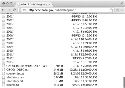
So, the main directory on the FTP site (/pub/data/gsod/) has a directory for each year that has the weather data. There's also a file called ish-history.csv. This contains information about the weather stations, when they were operational, and where they were located. (Also, the text files and README files are always important for more specific, detailed information about what's in each file.)
Now let's check out one of the data directories; this is for 2013.
The data directories contain a large number of data files. Each of the files that ends in .op.gz has three components for its file name. The first two parts are identifiers for the weather station and the third is the year.
Each data directory also has a tarball that contains all of the *.op.gz data files. That file will be the easiest to download, and then we can extract the *.op.gz files from it. Afterwards, we'll need to decompress these files to get the *.op data files. Let's do that, and then we can look at the data that we have.
Before we actually get into any of the code to do this, let's take a look at the dependencies that we'll need.
Before we get started, let's set up our project. For this chapter, our Leiningen 2 (http://leiningen.org/) project.clj file should look something like the following code:
(defproject clj-gis "0.1.0-SNAPSHOT"
  :dependencies [[org.clojure/clojure "1.5.1"]
                 [me.raynes/fs "1.4.4"]
                 [com.velisco/clj-ftp "0.3.0"]
                 [org.clojure/data.csv "0.1.2"]
                 [clj-time "0.5.1"]
                 [incanter/incanter-charts "1.5.1"]]
  :jvm-opts ["-Xmx4096m"])
Now for this section of code, let's open the src/clj_gis/download.clj file. We'll use this namespace declaration for this code as follows:
(ns clj-gis.download
  (:require [clojure.java.io :as io]
            [me.raynes.fs.compression :as compression]
            [me.raynes.fs :as fs]
            [miner.ftp :as ftp]
            [clj-gis.locations :as loc]
            [clj-gis.util :as u])
  (:import [org.apache.commons.net.ftp FTP]
           [java.util.zip GZIPInputStream]
           [java.io BufferedInputStream]))
Now, the next two functions together download the GSOD data files. The main function is download-data. It walks the directory tree on the FTP server, and whenever it identifies a file to be downloaded, it hands it off to download-file. This function figures out where to put the file and downloads it to that location. I've left out the source code for some of the utilities and secondary functions listed here, such as download-src, so that we can focus on the larger issues. You can find these functions in the file in this chapter's code download. The following code snippet is part of the code that is available for download:
(defn download-file
  "Download a single file from FTP into a download directory."
  [client download-dir dirname]
  (let [src (download-src dirname)
        dest (download-dest download-dir dirname)]
    (ftp/client-get client src dest)))

(defn download-data
  "Connect to an FTP server and download the GSOD data files."
  [uri download-dir data-dir]
  (let [download-dir (io/file download-dir)
        data-dir (io/file data-dir)]
    (ensure-dir download-dir)
    (ensure-dir data-dir)
    (ftp/with-ftp [client uri]
      (.setFileType client FTP/BINARY_FILE_TYPE)
      (doseq [dirname
              (filter get-year
                      (ftp/client-directory-names client))]
(download-file client download-dir dirname)))))Now, we've downloaded the files from the NOAA FTP server onto the local hard drive. However, we still need to use the tar utility to extract the files we've downloaded and then decompress them.
We'll use the FS library to extract the downloaded files. Currently, the individual data files are in a common Unix file format called tar, which collects multiple files into one larger file. These files are also compressed using the utility
gzip. We'll use Java's GZIPOutputStream to decompress gz. Let's see how this works:
(defn untar
  "Untar the file into the destination directory."
  [input-file dest-dir]
  (compression/untar input-file dest-dir))

(defn gunzip
  "Gunzip the input file and delete the original."
  [input-file]
  (let [input-file (fs/file input-file)
        parts (fs/split input-file)
        dest (fs/file (reduce fs/file (butlast parts))
                      (first (fs/split-ext (last parts))))]
    (with-open [f-in (BufferedInputStream.
                       (GZIPInputStream.
                         (io/input-stream input-file)))]
      (with-open [f-out (io/output-stream dest)]
        (io/copy f-in f-out)))))
We can put these functions together with the download functions that we just looked at. This function, download-all, will download all the data and then decompress all of the data files into a directory specified by clj-gis.locations/*data-dir*:
(defn download-all []
  (let [tar-dir (fs/file loc/*download-dir*)
        data-dir (fs/file loc/*data-dir*)]
    (download-data tar-dir data-dir)
    (doseq [tar-file (fs/list-dir tar-dir)]
      (untar (fs/file tar-dir tar-file) data-dir))
    (doseq [gz-file (fs/list-dir data-dir)]
      (gunzip (fs/file data-dir gz-file)))))
Now, what do these files look like? The header line of one of them is as follows:
STN--- WBAN YEARMODA TEMP DEWP SLP STP VISIB WDSP MXSPD GUST MAX MIN PRCP SNDP FRSHTT
The following is one of the data rows:
007032 99999 20130126 80.1 12 65.5 12 9999.9 0 9999.9 0 999.9 0 2.5 12 6.0 999.9 91.4* 71.6* 0.00I 999.9 000000
So, there are some identification fields, some for temperature, dew point, wind, and other weather data. Next, let's see how to winnow the data down to just the information that we plan to use.
As we just noticed, there's a lot of data in the GSOD files that we don't plan to use. This includes the following:
- Too many files with data for places that we aren't interested in
- Too many rows with data for months that we aren't interested in
- Too many columns with weather data that we aren't interested in (dew points, for instance)
At this point, we'll only worry about the first problem. Just filtering out the places we're not looking at will dramatically reduce the amount of data that we're dealing with from approximately 20 GB of data to just 3 GB.
The code for this section will be in the src/clj_gis/filter_data.clj file. Give it the following namespace declaration:
(ns clj-gis.filter-data
  (:require
    [clojure.string :as str]
    [clojure.data.csv :as csv]
    [clojure.java.io :as io]
    [me.raynes.fs :as fs]
    [clj-gis.locations :as loc]
    [clj-gis.util :refer (ensure-dir)]))
Now it's time for the code that is to be put in the rest of the file.
To filter out the data that we won't use, we'll copy files for stations in the United States into their own directory. We can create a set of these stations from the ish-history.csv file that we noticed earlier, so our first task will be parsing that file. This code will read the CSV file and put the data from each line into a new data record, IshHistory. Having its own data type for this information isn't necessary, but it makes the rest of the code much more readable. For example, we can reference the country field using (:country h) instead of (nth h 3) later. This type can also reflect the column order from the input file, which makes reading the data easier:
(defrecord IshHistory
  [usaf wban station_name country fips state call
   lat lon elevation begin end])
(defn read-history
  "Read the station history file."
  [filename]
  (with-open [f (io/reader filename)]
    (doall
      (->> (csv/read-csv f)
        (drop 1)
        (map #(apply ->IshHistory %))))))
The stations are identified by the combination of the USAF and WBAN fields. Some stations use USAF, some use WBAN, and some use both. So we'll need to track both to uniquely identify the stations. This function will create a set of the stations in a given country:
(defn get-station-set
  "Create a set of all stations in a country."
  [country histories]
  (set (map #(vector (:usaf %) (:wban %))
            (filter #(= (:country %) country)
                    histories))))
Finally, we need to tie these functions together. This function, filter-data-files, reads the history and creates the set of stations that we want to keep. Then, it walks through the data directory and parses the file names to get the station identifiers for each file. Files from the stations in the set are then copied to a directory with the same name as the country code, as follows:
(defn filter-data-files
  "Read the history file and copy data files matching the
  country code into a new directory."
  [ish-history-file data-dir country-code]
  (let [history (read-history ish-history-file)
        stations (get-station-set country-code history)]
    (ensure-dir (fs/file country-code))
    (doseq [filename (fs/glob (str data-dir "*.op"))]
      (let [base (fs/base-name filename)
            station (vec (take 2 (str/split base #"-")))]
        (when (contains? stations station)
          (fs/copy filename (fs/file country-code base)))))))
This set of functions will filter out most of the data and leave us with only the observations from the stations we're interested in.
We aren't plotting the raw data. Instead, we want to filter it further and summarize it. This transformation can be described in the following steps:
- Process only the observations for the month of July.
- Find the mean temperature for the observations for the month of July for each year, so we'll have an average for July 2013, July 2012, July 2011, and so on.
- Group these monthly averages into rolling ten-year windows. For example, one window will have the observations for 1950 to 1960, another window will have observations for 1951 to 1961, and so on.
- Find the mean temperature for each of these windows for a climatic average temperature for July for that period.
- Calculate the change in the maximum temperature by subtracting the climatic average for the last window for a station from the average of its first window.
This breaks down the rest of the transformation process pretty well. We can use this to help us structure and write the functions that we'll need to implement the process. However, before we can get into that, we need to read the data.
We'll read the data from the space-delimited data files and store the rows in a new record type. For this section, let's create the src/clj_gis/rolling_avg.clj file. It will begin with the following namespace declaration:
(ns clj-gis.rolling-avg
  (:require
    [clojure.java.io :as io]
    [clojure.string :as str]
    [clojure.core.reducers :as r]
    [clj-time.core :as clj-time]
    [clj-time.format :refer (formatter parse)]
    [clojure.data.csv :as csv]
    [me.raynes.fs :as fs]
    [clj-gis.filter-data :as fd]
    [clj-gis.locations :as loc]
    [clj-gis.types :refer :all]
    [clj-gis.util :as u]))
Now, we can define a data type for the weather data. We'll read the data into an instance of WeatherRow, and then we'll need to normalize the data to make sure that the values are ones that we can use. This will involve converting strings to numbers and dates, for instance:
(defrecord WeatherRow
  [station wban date temp temp-count dewp dewp-count slp
   slp-count stp stp-count visibility vis-count wdsp
   wdsp-count max-wind-spd max-gust max-temp min-temp
   precipitation snow-depth rfshtt])
(defn read-weather
  [filename]
  (with-open [f (io/reader filename)]
    (doall
      (->> (line-seq f)
        (r/drop 1)
        (r/map #(str/split % #"s+"))
        (r/map #(apply ->WeatherRow %))
        (r/map normalize)
        (r/remove nil?)
        (into [])))))
Now that we have the weather data, we can work it through the pipeline as outlined in the preceding code snippet. This series of functions will construct a sequence of reducers.
Reducers, introduced in Clojure 1.5, are a relatively new addition to the language. They refine traditional functional-style programming. Instead of map taking a function and a sequence and constructing a new sequence, the reducers' version of map takes a function and a sequence or folder (the core reducer data type) and constructs a new folder that will apply the function to the elements of the input when required. So, instead of constructing a series of sequences, it composes the functions into a larger function that performs the same processing, but only produces the final output. This saves on allocating the memory, and if the input data types are structured correctly, the processing can also be automatically parallelized as follows:
- For the first step, we want to return only the rows that fall in the month we're interested in. This looks almost exactly like a regular call to
filter, but instead of returning a new, lazy sequence, it returns a folder that has the same effect; it produces a sequence with only the data rows we want. Or, we can compose this with other folders to further modify the output. This is what we will do in the next few steps:(defn only-month "1. Process only the observations for the month of July." [month coll] (r/filter #(= (clj-time/month (:date %)) month) coll))
- This function takes the reducer from the first step and passes it through a few more steps. The
group-byfunction finally reifies the sequence into a hash map. However, it's immediately fed into another reducer chain that averages the accumulated temperatures for each month:(defn mean [coll] (/ (sum coll) (double (count coll)))) (defn get-monthly-avgs "2. Average the observations for each year's July, so we'll have an average for July 2013, one for July 2012, one for July 2011, and so on." [weather-rows] (->> weather-rows (group-by #(clj-time/year (:date %))) (r/map (fn [[year group]] [year (mean (map :max-temp group))])))) - For step three, we create a series of moving windows across the monthly averages. If there aren't enough averages to create a full window, or if there are only enough to create one window, then we throw those extra observations out:
(defn get-windows "3. Group these monthly averages into a rolling ten-year window. For example, one window will have the observations for 1950–1960. Another window will have observations for 1951–1961. And so on." [period month-avgs] (->> month-avgs (into []) (sort-by first) (partition period 1) (r/filter #(> (count %) 1)) (r/map #(vector (ffirst %) (map second %)))))) - This step uses a utility function,
mean, to get the average temperature for each window. We saw this defined in step two. This keeps hold of the starting year for that window so they can be properly ordered:(defn average-window "4. Average each of these windows for a climatic average temperature for July for that period." [windows] (r/map (fn [[start-year ws]] [start-year (mean ws)]) windows)) - After this, we do a little more filtering to only pass the averages through,and then we replace the list of averages with the difference between the initial and the final averages:
(defn avg-diff
  "5. Calculate the change in maximum temperature by
  subtracting the climatic average for the last window for
  a station from the average of its first window."
  [avgs]
  (- (last avgs) (first avgs)))
There's more to this, of course. We have to get a list of the files to be processed, and we need to do something with the output; either send it to a vector or to a file.
Now that we've made it this far, we're done transforming our data, and we're ready to start our analysis.
In the end, we're going to feed the data we've just created to ArcGIS in order to create the heat map, but before we do that, let's try to understand what will happen under the covers.
For this code, let's open up the src/clj_gis/idw.clj file. The namespace for this should be like the following code:
(ns clj-gis.idw
  (:require [clojure.core.reducers :as r]
            [clj-gis.types :refer :all]))
To generate a heat map, we first start with a sample of points for the space we're looking at. Often, this space is geographical, but it doesn't have to be. Values for a complex, computationally-expensive, two-dimensional function are another example where a heat map would be useful. It would take too long to completely cover the input domain, and inverse distance weighting could be used to fill in the gaps.
The sample data points each have a value, often labeled z to imply a third dimension. We want a way to interpolate the z value from the sample points onto the spaces between them. The heat map visualization is just the result of assigning colors to ranges of z and plotting these values.
One common technique to interpolate the value of z to points between the sample points is called inverse distance weighting (IDW). To find the interpolated value of z for a point x, y, IDW sees how much the value of each sample point influences that location, given each sample's distance away and a value p that determines how far each sample point's influence carries. Low values of p don't project much beyond their immediate vicinity. High values of p can be projected too far. We'll see some examples of this in a minute.
There are a variety of ways to calculate the IDW. One general form is to sum the weighted difference between the data point in question and all others, and divide it by the non-weighted sum.
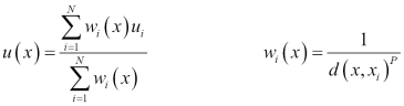
There are several variations of IDW, but here, we'll just describe the base version, as outlined by Donald Shepard in 1968. First, we have to determine the inverse distance function. It's given here as w. Also, x_i is the sample point, and x is the point to estimate the interpolation for, just as given in the preceding formula:
(defn w
  "Finds the weighted inverse distance between the points x and
  x_i. "
  ([p dist-fn x] (partial w p dist-fn x))
  ([p dist-fn x x_i]
   (/ 1.0 (Math/pow (dist-fn x x_i) p))))
With this in place, IDW is the sum of w for each point in the sample, multiplied by that sample point's value and divided by the sum of w for all the samples. It's probably easier to parse the code than it is to describe it verbosely:
(defn sum-over [f coll] (reduce + (map f coll)))
(defn idw
  ([sample-points data-key p dist-fn]
   (partial idw sample-points data-key p dist-fn))
  ([sample-points data-key p dist-fn point]
   (float
     (/ (sum-over #(* (w p dist-fn point %) (data-key %))
                  sample-points)
        (sum-over (w p dist-fn point) sample-points))))
  ([sample-points data-key p dist-fn lat lon]
   (idw sample-points data-key p dist-fn
        (->DataPoint lat lon nil))))
The highlighted part of the function is the part to pay attention to. The rest makes it easier to call idw in different contexts. I precompute the denominator in the let form, as it won't change for each sample point that is considered. Then, the distances of each sample point and the target point are multiplied by the value of each sample point and divided by the denominator, and this is summed together.
This function is easy to call with the charting library that Incanter provides, which has a very nice heat map function. Incanter is a library used to perform data analysis and visualization in Clojure by interfacing with high-performance Java libraries. This function first gets the bounding box around the data and pads it a little. It then uses Incanter's heat-map function to generate the heat map. To make it more useful, however, we then make the heat map transparent and plot the points from the sample onto the chart. This is found in src/clj_gis/heatmap.clj:
(defn generate-hm
  [sample p border]
  (let [{:keys [min-lat max-lat min-lon max-lon]}
        (min-max-lat-lon sample)]
    (->
      (c/heat-map (idw sample :value p euclidean-dist)
                  (- min-lon border) (+ max-lon border)
                  (- min-lat border) (+ max-lat border))
      (c/set-alpha 0.5)
      (c/add-points (map :lon sample) (map :lat sample)))))
Let's take a random data sample and use it to see what different values of p do.
For the first experiment, let's look at p=1:
(i/view (hm/generate-hm sample 1.0 5.0))
The graph it produces looks like the following figure:
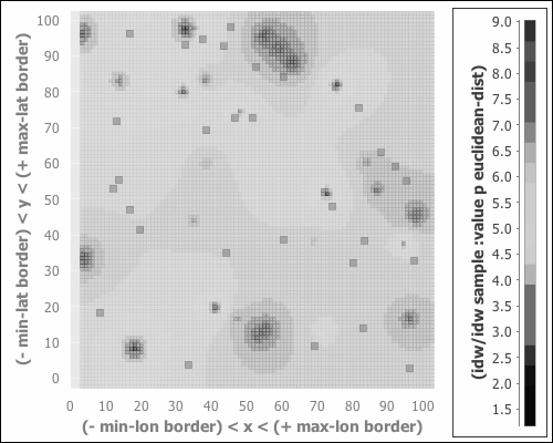
We can see that the influence for each sample point is tightly bound to its immediate neighborhood. More moderate values, around 4 and 5, dominate.
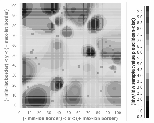
For p=8, the picture is a bit different, as shown in the following screenshot:
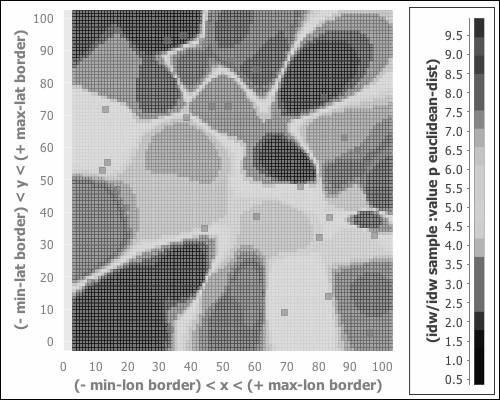
In the preceding figure, each interpolated point is more heavily influenced by the data points closest to it, and further points are less influential. More extreme regions have great influence over larger distances, except around sample points with moderate values.
Finally, we'll look at an interpolated point that's more balanced. The following is the chart for when p=3:
This seems much more balanced. Each sample point clearly exerts its influence across its own neighborhood. However, no point, and no range of values, appears to dominate. A more meaningful graph with real data would probably look quite good.
So far, we've been playing with the toy data. Before we can apply this to the climate data that we prepared earlier, there are several things we need to take into consideration.