
In this chapter, we'll look at Benford's Law; an interesting set of properties that are inherent in many naturally occurring sequences of numbers. For these sets of numbers, this observation predicts the distribution of initial digits.
The odd rule captures an interesting observation about the way numbers are distributed, and it's useful too. Benford's Law has been used as an evidence of fraud. If a sequence of numbers should be naturally occurring but Benford's Law indicates that they are not, then the sequence is likely to be fraudulent. For example, the daily balances in your bank account should follow Benford's Law, but if they don't, that may be evidence that someone is cooking the books.
Originally, Benford's Law was observed by the astronomer Simon Newcomb in 1881. He was referencing the logarithm tables, which were tomes listing the values for logarithms of different numbers. He noticed that the pages of the books were more worn out and discolored at the beginning than they were at the end. In fact, the pages that deal with numbers that begin with 1 were significantly more worn out than pages that begin with 9. As the initial digits climbed, the pages were less and less worn.
This phenomenon was noticed again in 1938 by the physicist Frank Benford. He tested this against data in a number of domains, and the principle now bears his name.
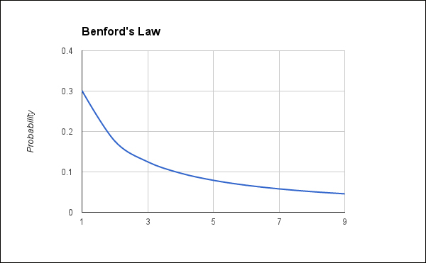
In practical terms, this means that about one-third of the numbers in the sequence begin with the digit 1, a little more than 15 percent begin with 2, about 12 percent begin with 3, and the rest until the digit 9 are all below 10 percent. Five percent of the numbers begin with 9. The following is a graphical representation of Benford's law:
So what's the logic behind this? Although the observation itself is surprising, understanding it is really not that difficult. Let's walk through an example to see what we can learn.
First, we'll take the example of putting a 100 dollars in the bank and earning an unheard-of 10 percent interest per year, compounded monthly, where the annual interest rate is divided evenly by the number of times it is compounded (in this case, 12), and that is the effective interest rate used each for compounding period. This behavior is evident in more typical interest rates too, but it takes a longer span of time. Let's look at a table of the end-of-year reports for this account:
|
Year |
Amount in dollars |
|---|---|
|
0 |
100.00 |
|
1 |
110.47 |
|
2 |
122.04 |
|
3 |
134.82 |
|
4 |
148.94 |
|
5 |
164.53 |
|
6 |
181.76 |
|
7 |
200.79 |
|
8 |
221.82 |
|
9 |
245.04 |
|
10 |
270.70 |
|
11 |
299.05 |
|
12 |
330.36 |
|
13 |
364.96 |
|
14 |
403.17 |
|
15 |
445.39 |
|
16 |
492.03 |
|
17 |
543.55 |
|
18 |
600.47 |
|
19 |
663.35 |
|
20 |
732.81 |
|
21 |
809.54 |
|
22 |
894.31 |
|
23 |
987.96 |
|
24 |
1,091.41 |
When the money in a bank account is compounded, the amount of money increases nonlinearly. That is, as the 0.30 dollars of interest that I accrued last month is now earning interest, this month, I'll earn 0.32 dollars. As each month's interest is rolled back into the balance, the amount increases faster and faster.
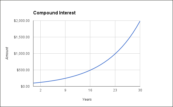
Looking at the balances, we can see that the amount stays in the 100s longer than it does in any other number (seven years). It only stays five years in the 200s. Finally, it stays in the 900s for only one year, at which point it rolls over, and the process starts all over again. Because there is less to work with and grow on, the lower the number (that is, in the 100s), the longer the graph will take to grow out of that range.
This pattern is common in any geometrically increasing amounts. Populations increase in this way, as do many other sequences.
However, concrete examples are always good. In this chapter, we'll work through several concrete examples. Then, we'll see what a failure of Benford's Law looks like, and finally, we'll look at an example of its use in life.
For the first illustration, let's keep working with the example we just started with.
There are good implementations of analyses using Benford's Law already in a number of libraries—we'll use Incanter (http://incanter.org/) for the examples later in the chapter—but to better understand what's going on, we'll write our own implementation first. To get started, the project.clj file for this chapter is as follows:
(defproject benford "0.1.0-SNAPSHOT"
  :dependencies [[org.clojure/clojure "1.5.1"]
                 [org.clojure/data.csv "0.1.2"]
                 [incanter "1.5.2"]])
The namespace declaration is as follows:
(ns benford.core
  (:require [clojure.string :as str]
            [clojure.java.io :as io]
            [clojure.pprint :as pp]
            [clojure.data.csv :as csv]
            [incanter.stats :as s]))
First, we need a way to take a sequence of numbers and pull the first digit out of each. There are a couple of ways to do this. We could do this mathematically by repeatedly dividing by ten until the value is less than ten. At that point, we take the integer portion of the result.
However, we'll do something simpler for this. We'll convert the number to a string and use a simple regular expression to skip over any signs or prefixes and just take the first digit. We'll convert that single digit back into an integer as follows:
(defn first-digit [n]
  (Integer/parseInt (re-find #"d" (str n))))
Now, extracting the first digits for each item in a sequence of numbers becomes simple:
(defn first-digit-freq [coll]
  (frequencies (map first-digit coll)))
Let's use these to pull the first digit from the yearly balances of the compound interest data, and we can graph them against the expected probabilities for Benford's Law.
The graph that is the result of this analysis is shown as follows. It looks at 25 years of accumulated interest, which is enough to go from 100 dollars to more than 1,000 dollars.
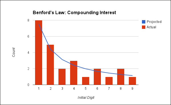
This gives us an idea of just how close the number sequence is. However, while the bars appear to match the line, they don't quite match. Are they close enough? We need to apply a simple statistical test to find out the answer.
First, we'll need a function that computes the expected value for sequences that conform to Benford's Law. This will take a digit and return the expected proportion for the number of times that digit starts the sequence:
(defn benford [d]
  (Math/log10 (+ 1.0 (/ 1.0 (float d)))))
We can use this to produce the full sequence of ratios for Benford's Law. We can see that the blue line in the preceding graph tracks the following values:
user=> (map benford (range 1 10))
(0.3010299956639812 0.17609125905568124 0.12493873660829993 0.09691001300805642 0.07918124604762482 0.06694678963061322 0.05799194697768673 0.05115252244738129 0.04575749056067514)
Next, we'll need a statistical function to test whether the frequencies of digits in a sequence match these values or not. As this is categorical data, Pearson's Χ2 (chi-squared) test is commonly used to test for conformance with Benford's Law.
The formula for the Χ2 test is simple. This uses O for the observed data and E for the expected data. N is the number of the categories of data. For example, numbers that begin with 1 are one category. In the case of testing against Benford's law, N will always be 9.
The formula for an Χ2 test looks like what is shown in the following figure:
This translates directly into Clojure. The only wrinkle here is that we need to compare the same quantities. This uses ratios for the expected values but raw frequencies for the observed data. So we take the total number of observations and scale the expected ratios to match it:
(defn x-sqr [expected-ratios observed]
  (let [total (sum observed)
        f (fn [e o]
            (let [n (- o e)]
              (/ (* n n) e)))]
    (sum (map f (map #(* % total) expected-ratios) observed))))
We can tie together the Χ2 function to the expected values from Benford's Law:
(defn benford-test [coll]
  (let [freqs (first-digit-freq coll)
        digits (range 1 10)]
    (x-sqr (map benford digits) (map freqs digits))))
Let's see what kind of results it gives out:
user=> (benford-test data)
1.7653767101950812
What does this number mean? The way this test is set up, values close to zero indicate that the sequence conforms to Benford's Law.
The value we obtained here, 1.8, is fairly close to zero, given the range of this function, so this looks good. However, we still need to know whether it's statistically significant or not. To find that, we need to find the p-value for this Χ2. There is the probability that this would happen by chance.
However, before we can find that information for an Χ2 test, we have to know the degrees of freedom in our experiment. This is the number of variables that are free to vary. Generally, for Χ2, the degree of freedom is one less than the number of cells in the test, so for Benford's Law, the degrees of freedom will be eight.
We use this information to find the value's probability of occurring in a Χ2 cumulative distribution. A cumulative distribution is the probability that a value or lesser value would occur. While a probability distribution gives the probability of x having a given value, a cumulative distribution gives the probability that x is less than or equal to that value. Incanter has a CDF for Χ2 in incanter.stats/cdf-chisq. We can use this to find p for any output of the Χ2 test:
user=> (s/cdf-chisq 1.7653 :df 8 :lower-tail? false)
0.9873810658453659
This is a very high p-value. We'd like it to be above 0.05; any value below that would indicate that this data did not follow Benford's law. (We'll get into the reasons for this in Chapter 7, Null Hypothesis Tests – Analyzing Crime Data when we discuss the null-hypothesis testing.) As it's higher, it's clear that this sequence of numbers tracks the predications of Benford's Law. There is no evidence of tampering here.
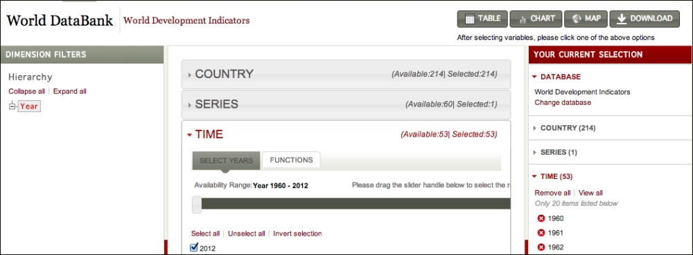
For the next example, let's look at the world population data. I downloaded this from World DataBank (http://databank.worldbank.org/). To download it to your computer, use the following steps:
- Navigate to the World Development Indicators database.
- Select all countries.
- Select Population (Total).
- Select all years.
- Click on Download and download the data as a CSV file.
- To make it easier to reference later, I moved and renamed this file
data/population.csv.
Now, let's read in this data. To make this easier, we'll write a function that reads in a CSV file, and from each row, create a map that uses the values from the header row as keys. The data for this looks like the following code snippet, which lists the header row and one data row:
Country Name,Country Code,Indicator Name,Indicator Code,1960 [YR1960],1961 [YR1961],1962 [YR1962],1963 [YR1963],1964 [YR1964],1965 [YR1965],1966 [YR1966],1967 [YR1967],1968 [YR1968],1969 [YR1969],1970 [YR1970],1971 [YR1971],1972 [YR1972],1973 [YR1973],1974 [YR1974],1975 [YR1975],1976 [YR1976],1977 [YR1977],1978 [YR1978],1979 [YR1979],1980 [YR1980],1981 [YR1981],1982 [YR1982],1983 [YR1983],1984 [YR1984],1985 [YR1985],1986 [YR1986],1987 [YR1987],1988 [YR1988],1989 [YR1989],1990 [YR1990],1991 [YR1991],1992 [YR1992],1993 [YR1993],1994 [YR1994],1995 [YR1995],1996 [YR1996],1997 [YR1997],1998 [YR1998],1999 [YR1999],2000 [YR2000],2001 [YR2001],2002 [YR2002],2003 [YR2003],2004 [YR2004],2005 [YR2005],2006 [YR2006],2007 [YR2007],2008 [YR2008],2009 [YR2009],2010 [YR2010],2011 [YR2011],2012 [YR2012],2013 [YR2013]

Afghanistan,AFG,Population (Total),SP.POP.TOTL,8774440,8953544,9141783,9339507,9547131,9765015,9990125,10221902,10465770,10729191,11015621,11323446,11644377,11966352,12273589,12551790,12806810,13034460,13199597,13257128,13180431,12963788,12634494,12241928,11854205,11528977,11262439,11063107,11013345,11215323,11731193,12612043,13811876,15175325,16485018,17586073,18415307,19021226,19496836,19987071,20595360,21347782,22202806,23116142,24018682,24860855,25631282,26349243,27032197,27708187,28397812,29105480,29824536,..
The first function for this is read-csv:
(defn read-csv [filename]
  (with-open [f (io/reader filename)]
    (let [[row & reader] (csv/read-csv f)
          header (map keyword
                      (map #(str/replace % space -) row))]
      (doall
        (map #(zipmap header %) reader)))))
From this, we can create another function that reads in the population file and pulls out all the year columns and returns all the populations for all countries for all years in one long sequence:
(defn read-databank [filename]
  (let [year-keys (map keyword (map str (range 1960 2013)))]
    (->> filename
      read-csv
      (mapcat #(map (fn [f] (f %)) year-keys))
      (remove empty?)
      (map #(Double/parseDouble %))
      (remove zero?))))
One of the problems with the Χ2 test is that it is very sensitive to the sample size. Small samples (less than 50) will almost always have a high p-value. Likewise, large samples incline toward low p-values. In general, samples between 100 and 2,500 observations are a good range, but even in this range, we can see some variance. It's easy to create a function that returns a random subset of a collection. The only problem with using it is that the value of the statistical tests is dependent on the nature of the sample returned. However, that is always the problem with samples:
(defn sample [coll k]
  (if (<= (count coll) k)
    coll
    (let [coll-size (count coll)]
      (loop [seen #{}]
        (if (>= (count seen) k)
          (map #(nth coll %) (sort seen))
          (recur (conj seen (rand-int coll-size))))))))
Now we can put all of this together. For the last example, we used our own functions to perform the Benford's test and the Χ2 on the output. This time, we'll use Incanter's function for this purpose from incanter.stats. This also looks up the p-value from the Χ2 distribution, so it's a bit handier than doing it in two steps:
user=> (def population (b/read-databank "data/population.csv"))
#'user/population
user=> (def pop-test (s/benford-test (b/sample population 100)))
#'user/pop-test
user=> (:X-sq pop-test)
7.926272852944953
user=> (:p-value pop-test)
0.4407050181730324
As the value of p is greater than 0.05, this appears to conform to Benford's Law. Graphing this makes the p-Benford's Law relationship clearer. If anything, this seems a better fit than the preceding compounding interest data:
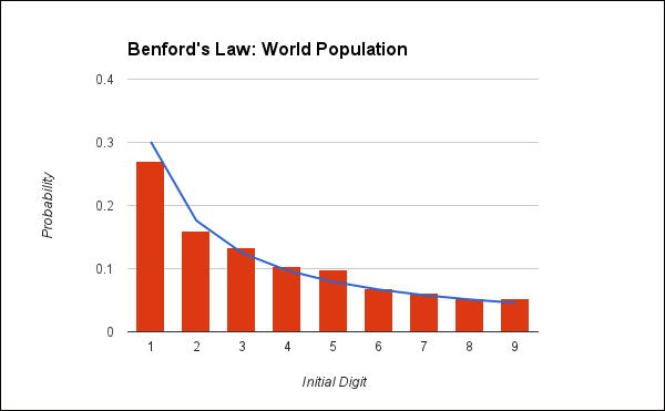
Again, it appears that this data also conforms to Benford's Law.