In this case, our hypothesis is that there is a relationship between the per capita gross national income and the rate of burglaries. We could go further and make the hypothesis stronger by specifying that higher GNI correlates to a higher burglary rate, somewhat counter-intuitively.

Given that statement of our working hypothesis, we can now formulate the null and alternative hypotheses.

These statements will now guide us through the rest of the process.

There are a number of assumptions in this data that we need to be aware of. First, since the crime data comes from multiple sources, there's going to be very little consistency in it.

To start with, the very definitions of these crimes may vary widely between different countries. Also, data collection procedures and practices will make the reliability of those numbers difficult.

The World Bank data is perhaps more consistent—things like land area can be measured and validated externally—but GNI can be reliant upon the own country's reporting, and that may often be inflated, as countries attempt to make themselves look more important and influential.

Moreover, there are also a lot of holes in the data. Because we haven't normalized the country names, there are no observations for the United States. It's listed as "United States" in one dataset and as "United States of America" in the other. And while this single instance would be simple to correct, we really have to do a more thorough audit of the country names.

So while there's nothing systematic that we need to take into account, there are several problems with the data that we need to keep in mind. We'll revisit these closer to the end of this chapter.

Now we have to determine which tests to run. Some tests are appropriate to different types of data and to different distributions of data. For example, nominal and numeric data require very different analyses.

If the relationship were known to be linear, we could use Pearson's correlation coefficient. Unfortunately, the relationship in our data appears to be more complicated than that.

In this case, our data is continuous numeric data. And we're interested in the relationship between two variables, but neither is truly independent, because we're not really sure exactly how the sampling was done, based on the description of the assumptions given earlier.

Because of all these factors, we'll use Spearman's rank correlation.

How did I pick this? It's fairly simple, but just complicated enough that we will not go into the details here.

The main point is that which statistical test you use is highly dependent on the nature of your data. Much of this knowledge comes from learning and experience, but once you've determined your data, a good statistical textbook or any of a number of online flowcharts can help you pick the right test.

But what is Spearman's rank correlation? Let's take a minute and find out.

Understanding Spearman's rank correlation coefficient

Spearman's rank correlation coefficient measures the association between two variables. It is particularly useful when only the rank of the data is known, but it can also be useful in other situations. For instance, it isn't thrown off by outliers, because it only looks at the rank.

The formula for this statistic is as follows:

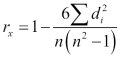
The value of n is the size of the sample. The value of d is each observation's difference in rank for the two variables. For example, in the data we've been looking at, Denmark ranks first for burglary (interesting), but third for per capita GNI. So Spearman's rank correlation would look at 3 – 1 = 2.

A coefficient of 0 means there is no relationship between the two variables, and a coefficient of -1 or +1 means that the two variables are perfectly related. That is, the data can be perfectly described using a monotonic function: a function from one variable to the other that preserves the order of the items. The function doesn't have to be linear. In fact, it could easily describe a curve. But it does capture the data.

The coefficient doesn't give us statistical significance (the p value), however. To get that, we just need to know that the Spearman's rank correlation coefficient is distributed approximately normally, when n ≥ 10. It has a mean of 0 and a standard deviation given as follows:

With these formulae, we can compute the z score of coefficient for our test. The z score is the distance of a data point from the mean, measured in standard deviations. The p value is closely related to the z score. So if we know the z score, we also know the p value.

Now we need to select how high of a bar we need the significance to rise to. The target p value is known as the α value. In general, α = 0.05 is commonly used, although if you want to be extra careful, α = 0.01 is also normal.

For this test, we'll just use α = 0.05.

We'll accept any kind of relationship for rejecting the null hypothesis, so this will be a two-tailed test. That means that the critical region will come from both sides of the curve, with their areas being 0.05 divided equally for 0.025 on each side.

This corresponds to a z score of z < -1.96 or z > 1.96.

We can use Incanter's function, incanter.stats/spearmans-rho, to calculate the Spearman's coefficient. However, it doesn't only calculate the z score. We can easily create the following function that wraps all of these calculations. We'll put this into src/nullh/stats.clj. We'll name the function spearmans.

(defn spearmans
  ([col-a col-b] (spearmans col-a col-b i/$data))
  ([col-a col-b dataset]
   (let [rho (s/spearmans-rho
               (i/sel dataset :cols col-a)
               (i/sel dataset :cols col-b))
         n (i/nrow dataset)
         mu 0.0
         sigma (Math/sqrt (/ 1.0 (- n 1.0)))
         z (/ (- rho mu) sigma)]
     {:rho rho, :n n, :mu mu, :sigma sigma, :z z})))

Now, we can run this on the dataset. Let's start from the beginning and load the datasets from the disk with the following commands:

user=> (def by-ny-gnp
         (d/load-join-pivot
           "unodc-data"
           "ny.gnp/ny.gnp.pcap.cd_Indicator_en_csv_v2.csv"))
#'user/by-ny-gnp
user=> (def burglary (d/by-crime by-ny-gnp "CTS 2012 Burglary"))
#'user/burglary
user=> (pprint (n-stat/spearmans :indicator-value :rate burglary))
{:rho 0.6938241467993876,
 :n 537,
 :mu 0.0,
 :sigma 0.04319342127906801,
 :z 16.063190325134588}

The preceding commands allowed us to see the process from front to back, and we can take the output and consider how the test went.

The final z-score was 16.03. Going by the book, a z-score this high is usually not even included on the charts. This would be a significant result, which would allow us to reject the null hypothesis. So, from this we can conclude that there is a relationship between the per capita GNI and the burglary rate.