The first step for analyzing a document, of course, is tokenizing. We'll use a simple tokenize function that just pulls out sequences of letters or numbers, including any single punctuation marks.

Now, we can use this function to see what words are present in the text and how frequent they are. The core Clojure function, frequencies, makes this especially easy, but we do still need to pull out the data that we'll use.

For each step, we'll first work on raw input, and then we'll write an additional utility function that modifies the :text property of the input NewsArticle.

To tokenize the text, we'll search for the matches for a regular expression and convert the output to lowercase. This won't work well for a lot of cases—contractions, abbreviations, and hyphenations in English, for example—but it will take care of simple needs. Look at the following code:

(defn tokenize [string]
  (map str/lower-case (re-seq #"[p{L}p{M}]+" string)))
(defn tokenize-text [m] (update-in m [:text] tokenize))

The actual tokenization is handled by the tokenize function. The tokenize-text function takes a NewsArticle instance and replaces its raw text property with the sequence of tokens generated from the text.

The function token-freqs replaces the sequence of tokens with a mapping of their frequencies. It uses the Clojure core function frequencies as shown in the following code:

(defn token-freqs [m] (update-in m [:text] frequencies))

We can then take a sequence of NewsArticle instances that contain the token frequencies and generate the frequencies for the entire corpus. The function corpus-freqs takes care of that. Look at the following code:

(defn corpus-freqs [coll]
  (reduce #(merge-with + %1 %2) {} (map :text coll)))

Let's use the following functions to get the frequencies:

We can see that the most frequent words are common words with little semantic value. In the next section, we'll see what we need to do with them.

The words identified as the most common words in the code in the previous section are often referred to as function words, because they're performing functions in the sentence, but not really carrying meaning. For some kinds of analyses, such as grammatical and stylistic analyses, these are vitally important. However, for this particular chapter, we're more interested in the documents' content words, or the words that carry semantic meaning.

To filter these out, the typical technique is to use a stop word list. This is a list of common words to remove from the list of tokens.

If you type english stop list into Google, you'll get a lot of workable stop lists. I've downloaded one from http://jmlr.org/papers/volume5/lewis04a/a11-smart-stop-list/english.stop. Download this file too, and place it into the d directory along with the data files.

To load the stop words, we'll use the following function. It simply takes the filename and returns a set of the tokens in it.

(defn load-stop-words [filename]
  (set (tokenize (slurp filename))))

Using this set directly is easy enough on raw strings. However, we'll want a function to make calling it on NewsArticle instances easier. Look at the following code:

(defn remove-stop-words [stop-words m]
  (update-in m [:text] #(remove stop-words %)))

Now, we can load those words and remove them from the lists of tokens. We'll start with the definition of tokens that we just created. Look at the following code:

user=> (def stop-words (nlp/load-stop-words "d/english.stop"))
user=> (def filtered
         (map #(nlp/remove-stop-words stop-words %) tokens))
user=> (take 10 (:text (first filtered)))
("harmonic" "convergences" "maxim" "strong" "point" "totally" "unsentimental" "ungenteel" "sendup" "model")

First, we can tell that we've removed a number of tokens that weren't really adding much. You, re, and s were all taken out, along with others.

Now let's regenerate the corpus frequencies with the following code:

user=> (def freqs (map nlp/token-freqs filtered))
user=> (def c-freqs (nlp/corpus-freqs freqs))
user=> (pprint (take 10 (reverse (sort-by second c-freqs))))
(["clinton" 8567]
 ["times" 6528]
 ["people" 6351]
 ["time" 6091]
 ["story" 5645]
 ["president" 5223]
 ["year" 4539]
 ["york" 4516]
 ["world" 4256]
 ["years" 4144])

This list seems much more reasonable. It focuses on Bill Clinton, who was the US President during this period.

Another way of dealing with this is to use a white list. This would be a set of words or features that represent the entire collection of those that we want to deal with. We could implement this as a simple function, keep-white-list, as shown in the following code:

(defn keep-white-list [white-list-set m]
  (over :text #(filter white-list-set %) m))

This function seems academic now, but we'll need it before we're done.

Now, let's look at a graph of the frequencies:

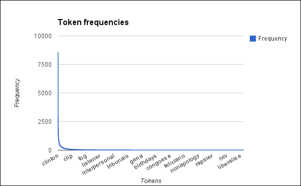
That's a lot of words that don't occur very much. This is actually expected. A few words occur a lot, but most just don't.

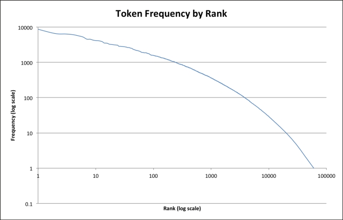
We can get another view of the data by looking at the log-log plot of the frequencies and ranks. Functions that represent a value raised to a power should be linear in these line charts. We can see that the relationship isn't quite on a line in this plot, but it's very close. Look at the following graph:

In fact, let's turn the frequency mapping around in the following code to look at how often different frequencies occur:

user=> (def ffreqs (frequencies (vals c-freqs)))
user=> (pprint (take 10 (reverse (sort-by second ffreqs))))
([1 23342]
 [2 8814]
 [3 5310]
 [4 3749]
 [5 2809]
 [6 2320]
 [7 1870]
 [8 1593]
 [9 1352]
 [10 1183])

So there are more than 23,000 words that only occur once and more than 8,000 words that only occur twice. Words like these are very interesting for authorship studies. The words that are found only once are referred to as hapax legomena, from Greek for "said once", and words that occur only twice are dis legomena.

Looking at a random 10 hapax legomena gives us a good indication of the types of words these are. The 10 words are: shanties, merrifield, cyberguru, alighting, roomfor, sciaretto, borisyeltsin, vermes, fugs, and gandhian. Some of these appear to be unusual or rare words. Others are mistakes or two words that were joined together for some reason, possibly by a dash.

Unfortunately, they do not contribute much to our study, since they don't occur often enough to contribute to the results statistically. In fact, we'll just get rid of any words that occur less than 10 times. This will form a second stop list, this time of rare words. Let's generate this list. Another, probably better performing, option is to create a whitelist of the words that aren't rare, but we can easily integrate this with our existing stop-list infrastructure, so we'll do it by just creating another list here.

To create it from the frequencies, we'll define a make-rare-word-list function. It takes a frequency mapping and returns the items with fewer than n occurrences, as follows:

(defn make-rare-word-list [freqs n]
  (map first (filter #(< (second %) n) freqs)))

We can now use this function to generate the d/english.rare file. We can use this file just like we used the stop list to remove items that aren't common and to further clean up the tokens that we'll have to deal with (you can also find this file in the code download for this chapter):

(with-open [f (io/writer "d/english.rare")]
  (binding [*out* f]
    (doseq [t (sort (nlp/make-rare-word-list c-freqs 8))]
      (println t))))

Now, we have a list of more than 48,000 tokens that will get removed. For perspective, after removing the common stop words, there were more than 71,000 token types.

We can now use that just like we did for the previous stop word list. Starting from filtered, which we defined in the earlier code after removing the common stop words, we'll now define filtered2 and recalculate the frequencies as follows:

user=> (def rare (nlp/load-stop-words "d/english.rare"))
user=> (def filtered2
         (map #(nlp/remove-stop-words rare %) filtered))
user=> (take 10 (:text (first filtered2)))
("maxim" "strong" "point" "totally" "unsentimental" "sendup" "model" "hustler" "difference" "surprise")

So we can see that the process has removed some uncommon words, such as harmonic and convergences.

This process is pretty piecemeal so far, but it's one that we would need to do multiple times, probably. Many natural language processing and text analysis tasks begin by taking a text, converting it to a sequence of features (tokenization, normalization, and filtering), and then counting them. Let's package that into one function as follows:

(defn process-articles
  ([articles]
   (process-articles
      articles ["d/english.stop" "d/english.rare"]))
  ([articles stop-files]
   (let [stop-words (reduce set/union #{}
                            (map load-stop-words stop-files))
         process (fn [text]
                   (frequencies
                     (remove stop-words (tokenize text))))]
     (map #(over :text process %) articles))))

The preceding function allows us to call it with just a list of articles. We can also specify a list of stop word files. The entries in all the lists are added together to create a master list of stop words. Then the articles' text is tokenized, filtered by the stop words, and counted. Doing it this way should save on creating and possibly hanging on to multiple lists of intermediate processing stages that we won't ever use later.

Now we can skip to the document-level frequencies with the following command:

user=> (def freqs (nlp/process-articles articles))

Now that we've filtered these out, let's look at the graph of token frequencies again:

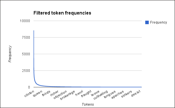
The distribution stayed the same, as we would expect, but the number of words should be more manageable.

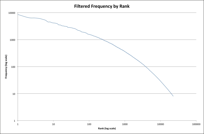
Again, we can see from the following log-log plot that the previous power relationship—almost, but not quite, linear—holds for this frequency distribution as well:

Another way to approach this would be to use a whitelist, as we mentioned earlier. We could load files and keep only the tokens that we've seen before by using the following function:

(defn load-articles [white-list-set articles]
  (let [process (fn [text]
                  (frequencies
                    (filter white-list-set (tokenize text))))]
    (map #(over :text process %) articles)))

Again, this will come up later. We'll find this necessary when we need to load unseen documents to analyze.

The frequencies as we currently have them will present a couple of difficulties. For one thing, if we have a document with 100 words and one with 500 words, we can't really compare the frequencies. For another thing, if a word occurs three times in every document, say in a header, it's not as interesting as one that occurs in only a few documents three times and nowhere else.

In order to work around both of these, we'll use a metric called term frequency-inverse document frequency (TF-IDF). This combines some kind of document-term frequency with the log of the percentage of documents that contain that term.

For the first part, term frequency, we could use a number of metrics. We could use a boolean 0 or 1 to show absence or presence. We could use the raw frequency or the raw frequency scaled. In this case, we're going to use an augmented frequency that scales the raw frequency by the maximum frequency of any word in the document. Look at the following code:

(defn tf [term-freq max-freq]
  (+ 0.5 (/ (* 0.5 term-freq) max-freq)))
(defn tf-article [article term]
  (let [freqs (:text article)]
    (tf (freqs term 0) (reduce max 0 (vals freqs)))))

The first function in the preceding code, tf, is a basic augmented frequency equation and takes the raw values as parameters. The second function, tf-article, wraps tf but takes a NewsArticle instance and a word and generates the TF value for that pair.

For the second part of this equation, the inverse document frequency, we'll use the log of the total number of documents divided by the number of documents containing that term. We'll also add one to the last number to protect against division-by-zero errors.

The idf function calculates the inverse document frequency for a term over the given corpus, as shown in the following code:

(defn has-term?
  ([term] (fn [a] (has-term? term a)))
  ([term a] (not (nil? (get (:text a) term)))))
(defn idf [corpus term]
  (Math/log
    (/ (count corpus)
       (inc (count (filter (has-term? term) corpus))))))

The IDF for a word won't change between different documents. Because of this, we can calculate all of the IDF values for all the words represented in the corpus once and cache them. The following two functions take care of this scenario:

(defn get-vocabulary [corpus]
  (reduce set/union #{} (map #(set (keys (:text %))) corpus)))
(defn get-idf-cache [corpus]
  (reduce #(assoc %1 %2 (idf corpus %2)) {}
          (get-vocabulary corpus)))

The first function in the preceding code, get-vocabulary, returns a set of all the words used in the corpus. The next function, get-idf-cache, iterates over the vocabulary set to construct a mapping of the cached IDF values. We'll use this cache to generate the TF-IDF values for each document.

The tf-idf function combines the output of tf and idf (via get-idf-cache) to calculate the TF-IDF value. In this case, we simply take the raw frequencies and the IDF value and multiply them together as shown in the following code:

(defn tf-idf [idf-value freq max-freq]
  (* (tf freq max-freq) idf-value))

This works at the most basic level; however, we'll want some adapters to work with NewsArticle instances and higher-level Clojure data structures.

The first level up will take the IDF cache and a map of frequencies and return a new map of TF-IDF values based off of those frequencies. To do this, we have to find the maximum frequency represented in the mapping. Then we can calculate the TF-IDF for each token type in the frequency map as follows:

(defn tf-idf-freqs [idf-cache freqs]
  (let [max-freq (reduce max 0 (vals freqs))]
    (into {}
          (map #(vector (first %)
                        (tf-idf
                          (idf-cache (first %))
                          (second %)
                          max-freq))
               freqs))))

The tf-idf-freqs function does most of the work for us. Now we can build on it further. First, we'll write tf-idf-over to calculate the TF-IDF values for all the tokens in a NewsArticle instance. Then we'll write tf-idf-cached, which takes a cache of IDF values for each word in a corpus. It returns those documents with their frequencies converted if TF-IDF. Finally, tf-idf-all will call this function on a collection of NewsArticle instances as shown in the following code:

(defn tf-idf-over [idf-cache article]
  (over :text (fn [f] (tf-idf-freqs idf-cache f)) article))
(defn tf-idf-cached [idf-cache corpus]
  (map #(tf-idf-over idf-cache %) corpus))
(defn tf-idf-all [corpus]
  (tf-idf-cached (get-idf-cache corpus) corpus))

We've implemented TF-IDF, but now we should play with it some more to get a feel for how it works in practice.

We'll start with the definition of filtered2 that we implemented in the Hapax and Dis Legomena section. This section contained the corpus of NewsArticles instances, and the :text property is the frequency of tokens without the tokens from the stop word lists of both rare and common words.

Now we can generate the scaled TF-IDF frequencies for these articles by calling tf-idf-all on them. Once we have that, we can compare the frequencies for one article. Look at the following code:

(def tf-idfs (nlp/tf-idf-all filtered2))
(doseq [[t f] (sort-by second (:text (first filtered2)))]
  (println t 	ab f 	ab (get (:text (first tf-idfs)) t)))

The table's too long to reproduce here (176 tokens). Instead, I'll just pick 10 interesting terms to look at more closely. The following table includes not only each term's raw frequencies and TF-IDF scores, but also the number of documents that they are found in:

The tokens in the preceding table are ordered by their raw frequencies. However, notice how badly that correlates with the TF-IDF.

What we wind up with is a measure of how important a term is in that document. Words that are more common have to appear more to be considered significant. Words that are found in only a few documents can be important with just one mention.

As a final step before we move on, we can also write a utility function that loads a set of articles, given a token whitelist and an IDF cache. This will be important }after we've trained the neural network when we're actually using it. That's because we will need to keep the same features, in the same order, and to scale between the two runs. Thus, it's important to scale by the same IDF values. Look at the following code:

(defn load-text-files [token-white-list idf-cache articles]
  (tf-idf-cached idf-cache
                 (load-articles token-white-list articles)))

The preceding code will allow us to analyze documents and actually use our neural network after we've trained it.