As the name implies, artificial neural networks are machine learning structures modeled on the architecture and behavior of neurons, such as the ones found in the human brain. Artificial neural networks come in many forms, but today we're going to use one of the oldest and most common forms: the three-layer feed-forward network.

We can see the structure of a unit outlined in the following figure:

Each unit is able to realize linearly separable functions. That is, functions that divide their n-dimensional output space along a hyperplane. To emulate more complex functions, however, we have to go beyond a single unit and create a network of them.

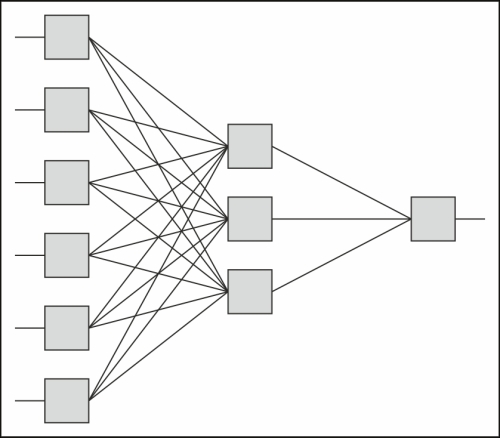
These networks have three layers: an input layer, a hidden layer, and an output layer. Each layer is made up of one or more neurons. Each neuron takes one or more inputs and produces an output, which is broadcast to one or more outputs. The inputs are weighted, and each input is weighted individually. All of the inputs are added together, and the sum is passed through an activation function that normalizes and scales the input. The inputs are x, the weights are w, and the outputs are y.

A simple schematic of this structure is shown as follows:

The network operates in a fairly simple manner, following the process called feed forward activation. It is described as follows:

Initially, the weights are usually randomly selected. Then the weights are trained using a variety of techniques. A common one is called backward propagation. This involves computing the error between the output neurons and the desired outputs. This error is then fed backward into the network. This is used to dampen some weights and increase others. The net effect is to nudge the output of the network slightly closer to the target.

Other training methods work differently, but attempt to do the same thing: each tries to modify the weights so that the outputs are close to the targets for each input in the training set.

Note that I said close to the targets. When training a neural network, you don't want the outputs to align exactly. When this happens, the network is said to have memorized the training set. This means that the network will perform great for inputs that it has seen previously. But when it encounters new inputs, it is brittle and won't perform well. It has learned the training set too well, but it won't be able to generalize that information to new inputs.

Implementing neural networks isn't difficult—and doing so is a useful exercise—but there are good libraries for neural networks available for Java and Clojure, and we'll choose one of those here. For our case, we'll use the Encog Machine Learning Framework (http://www.heatonresearch.com/encog), which specializes in neural networks. But we'll primarily be using it through the Clojure wrapper library Enclog (https://github.com/jimpil/enclog/). We'll build on these to write some facade functions over Enclog to customize this library for our processes.

The first step is to create the neural network. The make-network function takes the vocabulary size and the number of hidden nodes (the variables for our purposes), but it defines the rest of the parameters internally, as follows:

(defn make-network [vocab-size hidden-nodes]
  (nnets/network (nnets/neural-pattern :feed-forward)
                 :activation :sigmoid
                 :input (+ vocab-size (count periods))
                 :hidden [hidden-nodes]
                 :output 1))

The number of input nodes is a function of the size of the vocabulary in addition to the number of periods. (Periods is a non-dynamic, namespace-level binding. We may want to rethink that and make it dynamic to provide a little more flexibility, but for our needs right now this is sufficient.) And since from the output node, we just want a single value indicating whether the stock went up or down, we hardcoded the number of output nodes to one. However, the number of hidden nodes that will perform best is an open question. We'll include that as a parameter so we can experiment with it.

For the output, we'll need a way to take our expected output and run it through the same activation function as that output. That way, we can directly compare the two as follows:

(defn activated [act-fn output]
  (let [a (double-array 1 [output]))]
    (.activationFunction act-fn a 0 1)
    a)

The activated function takes an object that implements org.encog.engine.network.activation.ActivationFunction. We can get these from the neural network. It then puts the output for a period into a double array. The activation function scales this and then returns the array.

We will also need to prepare the data and insert it into a data structure that Encog can work with. The primary transformation in the following code is pulling out the output prices for the period that we're training for:

(defn build-data [nnet period training-set]
  (let [act (.getActivation nnet (dec (.getLayerCount nnet)))
        output (mapv #(activated act (get (:outputs %) period))
                     training-set)]
    (training/data :basic-dataset
                   (mapv :input training-set)
                   output)))

There's nothing particularly exciting here. We pull the inputs and the outputs for one time period out into two separate vectors and create a dataset with them.

Now we have a neural network, but it's been initialized to random weights, so it will perform very, very poorly. We'll need to train it immediately.

To do this, we will put the training set together with the network in the following code. Like the previous functions, train-for accepts the parameters that we're interested in being able to change, uses reasonable defaults for ones that we'll probably leave alone, but hardcodes parameters that we won't touch. The function creates a trainer object and calls its train method. Finally, we return the neural network, which was modified in place.

(defn train-for
  ([nnet period training-set]
    (train-for nnet period training-set 0.01 500 []))
  ([nnet period training-set error-tolerance
    iterations strategies]
    (let [data (build-data nnet period training-set)
          trainer (training/trainer :back-prop
                                    :network nnet:training-set data)]
      (training/train
        trainer error-tolerance iterations strategies)
      nnet)))

When it is time to validate a network, it will be a little easier to combine creating a network with training it into one function. We'll do that with make-train as follows:

(defn make-train [vocab-size hidden-count period coll]
  (let [nn (make-network vocab-size hidden-count)]
    (train-for nn period coll 0.01 100 [])
    nn))

This allows us to train a new neural network in one call.

Once we've trained the network, we'll want to run it on new inputs, ones for which we don't know the expected output. We can do that with the run-network function. This takes a trained network and an input collection and returns an array of the network's output as follows:

(defn run-network [nnet input]
  (let [input (double-array (count input) input)
        output (double-array (.getOutputCount nnet))]
    (.compute nnet input output)
    output))

We can use this function in one of two ways:

We'll see an example of the latter in the next section.

We can build on all of these functions to validate the neural network, train it, test it against new data, and evaluate how it does.

The test-on utility gets the sum of squared errors (SSE) for running the network on a test set for a given period. This trains and runs a neural network on the training set for a given period. It then returns the SSE for that run as follows:

(defn test-on [nnet period test-set]
  "Runs the net on the test set and calculates the SSE."
  (let [act (.getActivation nnet (dec (.getLayerCount nnet)))
        sqr (fn [x] (* x x))
        error (fn [{:keys [input outputs]}]
                (- (first (activated act (get outputs period)))
                   (first (run-network nnet input))))]
    (reduce + 0.0 (map sqr (map error test-set)))))

Running this train-test combination once gives us a very rough idea of how the network will perform with those parameters. However, if we want a better idea, we can use K-fold cross-validation. This divides the data into K equally sized groups. It then runs the train-test combination K times. Each time, it holds out a different partition as a test group. It trains the network on the rest of the partitions and evaluates it on the test group. The errors returned by test-on can be averaged to get a better idea of how the network will perform with those parameters.

For example, say we use K=4. We'll divide the training input into four groups: A, B, C, and D. This means that we'll train the following four different classifiers:

For each classifier, we'll compute the SSE, and we'll take the mean of these to see how well the classification should perform with those parameters, on average.

The x-validate function will perform the cross validation on the inputs. The other function, accum, is simply a small utility that accumulates the error values into a vector. The v/k-fold function expects the accumulator to return the base case (an empty vector) when called with no arguments, as shown in the following code:

(defn accum
  ([] [])
  ([v x] (conj v x)))
(defn x-validate [vocab-size hidden-count period coll]
  (v/k-fold #(make-train vocab-size hidden-count period %)
            #(test-on %1 period %2)
            accum
            10
            coll))

The x-validate function uses make-train to create a new network and train it. It tests that network using test-on, and it gathers the resulting error rates together with accum.

We've defined this system to let us play with a couple of parameters. First, we can set the number of neurons in the hidden layer. Also, we can set the time period that we are to predict for into the future (one day, two days, three days, a month, a year, and so on).

These parameters create a large space of possible solutions, some of which may perform better than others. We can make some educated guesses about some of the parameters—that it will predict the movement of the stock prices one day in the future better than it will the movement a year in the future—but we don't know that, and we should perhaps try it out.

These parameters present a search space. It would take too much time to try all the combinations, but we can try a number of them, just to see how they perform. This lets us tune the neural network to get the best results.

To explore this search space, let's first define what happens when we test one point, one combination of time period in the future, and a number of hidden nodes. The explore-point function will take care of this in the following code:

(defn explore-point [vocab-count period hidden-count training]
  (println period hidden-count)
  (let [error (x-validate
                vocab-count hidden-count period training)]
    (println period hidden-count
             '=> 	ab (u/mean error) 	ab error)
    (println)
    error))

The preceding code basically just takes the information and passes it to x-validate. It returns that function's return value (error) too. Along the way, it prints out a number of status messages. Then we need something that walks over the search space, calls explore-point, and collects the error rates returned for the output.

We'll define a dynamic global called *hidden-counts* that defines the range of hidden neuron counts that we're interested in exploring. The periods value that we bound earlier will define the search space for how far to look into the future.

To make sure that we don't train the networks too specifically on the data that we're using to find the best parameters, we'll first break the data into a development set and a test set. We'll use the development set to try out the different parameters, further breaking it up into a training set and a development-test set. At the end, we'll take the best set of parameters and test those against the test set that we originally held out. This will give us a better idea of how the neural network performs. The final-eval function will perform this last set and return the information that it creates.

The following function walks over these values and is named explore-params:

(def ^:dynamic *hidden-counts* [5 10 25 50 75])
(defn final-eval [vocab-size period hidden-count
                  training-set test-set]
  (let [nnet (make-train
               vocab-size hidden-count period training-set)
        error (test-on nnet period test-set)]
    {:period period
     :hidden-count hidden-count
     :nnet nnet
     :error error}))

(defn explore-params
  ([error-ref vocab-count training]
   (explore-params
     error-ref vocab-count training *hidden-counts* 0.2))
  ([error-ref vocab-count training hidden-counts test-ratio]
   (let [[test-set dev-set] (u/rand-split training test-ratio)
         search-space (for [p periods, h hidden-counts] [p h])]
     (doseq [pair search-space]
       (let [[p h] pair,
             error (explore-point vocab-count p h dev-set)]
         (dosync
           (commute error-ref assoc pair error))))
     (println "Final evaluation against the test set.")
     (let [[period hidden-count]
           (first (min-key #(u/mean (second %)) @error-ref))
           final (final-eval
                   vocab-count period hidden-count
                   dev-set test-set)]
       (dosync
         (commute error-ref assoc :final final))))
   @error-ref))

I've made a slightly unusual design decision in writing explore-params. Instead of initializing a hash map to contain the period-hidden count pairs and their associated error rates, I need the caller to pass in a reference containing a hash map. During the course of the processing, explore-params fills the hash map and finally returns it.

I've done this for one reason: exploring this search space still takes a long time. Over the course of writing this chapter, I needed to stop the validation, tweak the possible parameter values, and start it again. Setting up the function this way allowed me to be able to stop the processing, but still have access to what's happened thus far. I can look at the values, play around with them, and allow a more thorough examination of them to influence my decisions about what direction to take.