
18
Customizing the Render Pipeline
In Chapter 5, Let’s Light It Up!, we discussed adding color, textures, and lights to a scene. In our project, we colored vertices, applied textures, and turned on lights with single OpenGL calls.
Now in this chapter we will investigate how the color of all pixels is calculated through the use of shaders. When working with shaders, all the mathematics is revealed. With a few modifications to your project, by the end of this chapter you will be using shaders for the following purposes:
- Coloring and texturing mesh faces
- Turning on the lights
We will begin by grabbing the UV values that come with the OBJ model file and passing these values and a texture to a vertex and fragment shader for processing. This will allow us to color a model using an external image. Following this, because a plain image on a model will look rather flat, we’ll examine the fundamental lighting models that have been traditionally used to emulate lighting in graphics. Taking the mathematics from these models, we will translate them into shader code to light up the 3D scene.
Being able to understand mathematical concepts related to the calculations used in rendering and translating them into shader code is an essential skill for today’s graphics programmers. From this chapter, you will be able to examine theoretical concepts and implement them in your projects to extend the rendering possibilities.
Technical requirements
The solution files containing this chapter’s code can be found on GitHub at https://github.com/PacktPublishing/Mathematics-for-Game-Programming-and-Computer-Graphics/tree/main/Chapter1 8 in the Chapter18 folder.
Coloring and texturing mesh faces
Thus far, in our OpenGL project, we have implemented simple white mesh rendering. Now, it’s time to add the functionality of coloring and texturing polygons and pixels. The logic is similar to that of vertex coloring and UV mapping, as discussed in Chapter 5, Let’s Light It Up! Though now, when using shaders to do the rendering, the colors are added vertex by vertex and pixel by pixel.
A color is allocated to a vertex via the vertex shader and then passed to the fragment shader. The color for each vertex will specify the color of the pixel representing the vertex, but not the colors in between. Take, for example, the close-up of our teapot model in Figure 18.1:
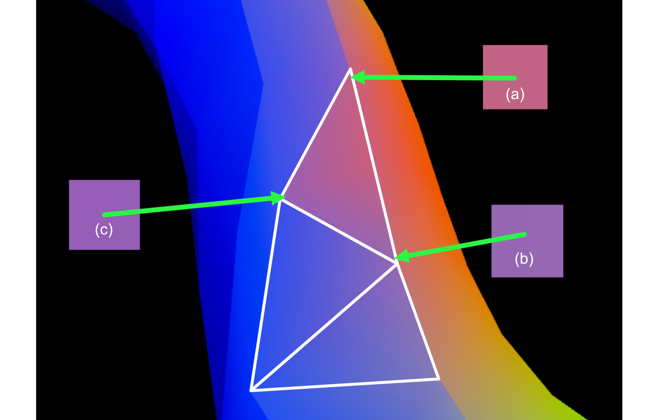
Figure 18.1: Polygons colored using vertex colors
The colors for each vector are indicated by (a), (b), and (c). This means the fragment shader must interpret what the value for each pixel between the vertices will be. As you can see from Figure 18.1, the colors fade from one vertex color to the other and across the polygon’s face. This is a blending or averaging across the surface and is calculated by the graphics card. By the time the color value is used in the fragment shader, it has become an interpolated blend of the vertex colors that surround it. You do not need to do any extra calculations.
To see this process of color blending, we will modify our project so that it uses vertex colors to color each polygon in the teapot model.
Let’s do it…
In this exercise, we will modify the project so that it colors the vertices of the teapot using the vertex normals. The project is already loading these normals from the mesh file, so only minimal changes need to be made:
- Make a copy of the Chapter_17 folder and name it Chapter_18.
- First, we need to modify LoadMesh.py to pass the vertex normal information that’s being extracted from the OBJ file to the vertex shader. Modify the code like so:
class LoadMesh(Mesh3D):
def __init__(self, vao_ref, material, draw_type,model_filename, texture_file=””,back_face_cull=False):self.coordinates =self.format_vertices(self.vertices, self.triangles)self.normals =self.format_vertices(self.normals,self.normal_ind)..
position = GraphicsData(“vec3”,self.coordinates)position.create_variable(material.program_id,“position”)vertex_normals = GraphicsData(“vec3”,self.normals)vertex_normals.create_variable(material.program_id,“vertex_normal”)def format_vertices(self, coordinates, triangles):..
We begin by reformatting the normals according to triangle order, as we had to do with the vertices in Chapter 17, Vertex and Fragment Shading.
Notice the new code for passing the normals to the shader is similar to that for passing the vertex positions. The difference is that the variable being created is called vertex_normal. This is exactly how it needs to be spelled in the vertex shader to ensure the data is passed correctly.
- Next, we must modify vertexcolvert.vs so that it accepts the vertex normal value and passes it onto the fragment shader:
#version 330 core
in vec3 position;
in vec3 vertex_normal;
uniform mat4 projection_mat;
uniform mat4 view_mat;
uniform mat4 model_mat;
out vec3 normal;
void main()
{gl_Position = projection_mat *inverse(transpose(view_mat)) *transpose(model_mat) *vec4(position, 1);normal = mat3(transpose(model_mat)) *vertex_normal;}
Here, the vertex normal is presented as an incoming vec3 value. Because this value is being passed out of the vertex shader, it needs to be given an output variable declared as out vec3 normal.
Inside the main() function, the normal is transformed into model space, which will allow it to take on transformations applied to the model.
- Now, we can modify vertexcolfrag.vs so that it uses the normal color for coloring fragments:
#version 330 core
in vec3 normal;
out vec4 frag_color;
void main()
{frag_color = vec4(normal, 1);}
Note that this normal is passed from the vertex shader as an in variable and then used to replace the white color we were previously using in Chapter 17, Vertex and Fragment Shading.
- A few tweaks in ShaderTeapot.py will make the starting render easier to examine. Modify this file like this:
mat = Material(“shaders/vertexcolvert.vs”,
“shaders/vertexcolfrag.vs”)quat_teapot.add_component(LoadMesh(
quat_teapot.vao_ref, mat,GL_TRIANGLES,“models/teapot.obj”))quat_teapot.add_component(mat)
quat_trans: Transform =
quat_teapot.get_component(Transform)quat_trans.update_position(pygame.Vector3(0, -1.5,
-5))quat_trans.rotate_y(90, False)
objects_3d.append(quat_teapot)
These changes allow the teapot to be fully rendered using GL_TRIANGLES. The position and rotation of the teapot have also been modified so that it appears nicely in the window when the program is run, as shown in Figure 18.2:
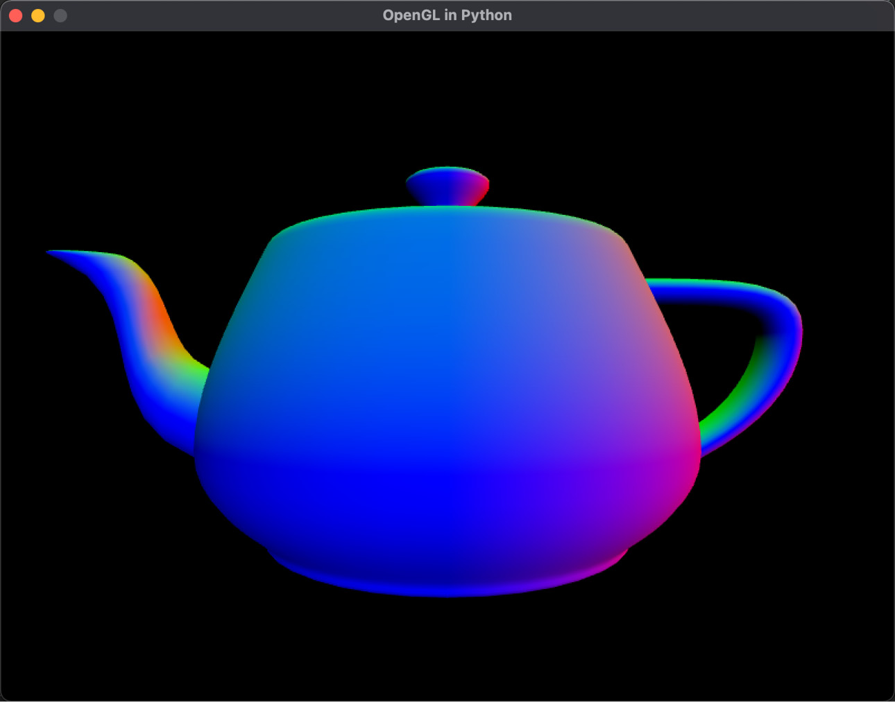
Figure 18.2: A vertex-colored teapot
- Run the ShaderTeapot.py file now to see the results.
In this exercise, you modified the project to draw a mesh as a solid object using GL_TRIANGLES, and also used normals to color the vertices. Next, we will modify the project and shaders to put a texture onto the teapot.
Just like the legacy version of OpenGL, shaders also require UV values to paste a texture onto the surface of a mesh. And just like vertex coloring, it’s only the vertices that have the UVs specified for them. The graphics card has to perform the same calculation it does for blending color across the surface of a polygon for UV values. The result is that a texture is stretched across the polygon, ensuring the UV values specified by the vertices end up with the associated UV value location in the texture. The UV values have already been extracted with the code for the OBJ file. Now, it’s time to put them into practice and texture the teapot.
Let’s do it…
In this exercise, we will feed the UV values from the OBJ file and a texture through to the shader to map a surface image onto the teapot:
- Create a new Python script called Texture.py. Add the following code:
import pygame
from OpenGL.GL import *
class Texture():
def __init__(self, filename=None):self.surface = Noneself.texture_id = glGenTextures(1)if filename is not None:self.surface = pygame.image.load(filename)self.load()
The initialization of the class sets up a surface to hold the data from an image file, which can be in PNG or TIF format. texture_id has been set up as a pointer to where this texture will be in memory and used by OpenGL to access and use the pixel colors.
The load() method formats the data from the image file into a format suitable for use by OpenGL:
    def load(self):
        width = self.surface.get_width()
        height = self.surface.get_height()
        pixel_data =
            pygame.image.tostring(self.surface,
                                  “RGBA”, 1)
        glBindTexture(GL_TEXTURE_2D, self.texture_id)
        glTexImage2D(GL_TEXTURE_2D, 0, GL_RGBA, width,
                     height, 0, GL_RGBA,
                     GL_UNSIGNED_BYTE, pixel_data)
        glGenerateMipmap(GL_TEXTURE_2D)
        glTexParameteri(GL_TEXTURE_2D,
                        GL_TEXTURE_MAG_FILTER,
                        GL_LINEAR)
        glTexParameteri(GL_TEXTURE_2D,
                        GL_TEXTURE_MIN_FILTER,
                        GL_LINEAR_MIPMAP_LINEAR)
        glTexParameteri(GL_TEXTURE_2D,
                        GL_TEXTURE_WRAP_S,
                        GL_REPEAT)
        glTexParameteri(GL_TEXTURE_2D,
                        GL_TEXTURE_WRAP_T,
                        GL_REPEAT)
You will notice a glBindTexture() call, which assigns texture_id as the location in memory where the data will be placed. Let’s explain these OpenGL calls:
- glTexImage2D(): Specifies the texture’s size and format. Go to https://registry.khronos.org/OpenGL-Refpages/gl4/html/glTexImage2D.xhtml for a full description.
- glGenerateMipmap(): Generates mipmaps for the texture. These are a series of lesser-resolution copies of the texture that can be used when the camera is far away from the object, thus making the surface appear blurry and far away. Go to https://registry.khronos.org/OpenGL-Refpages/gl4/html/glGenerateMipmap.xhtml for a full description.
- glTexParameteri(): Sets the parameters by which OpenGL will render the texture. Go to https://registry.khronos.org/OpenGL-Refpages/gl4/html/glTexParameter.xhtml for a full description.
- LoadMesh.py will need to be modified so that it passes a texture through to the shader:
from Mesh3D import *
from GraphicsData import *
from Uniform import *
from Texture import *
from Utils import *
class LoadMesh(Mesh3D):
def __init__(self, vao_ref, material, draw_type,model_filename, texture_file=””,back_face_cull=False):self.vertices, self.uvs,self.uvs_ind, self.normals,self.normal_ind, self.triangles =self.load_drawing(model_filename)self.coordinates = self.format_vertices(self.vertices, self.triangles)self.normals = self.format_vertices(self.normals, self.normal_ind)self.uvs = self.format_vertices(self.uvs, self.uvs_ind)self.draw_type = draw_typeself.material = material..
vertex_normals.create_variable(material.program_id,“vertex_normal”)v_uvs = GraphicsData(“vec2”, self.uvs)v_uvs.create_variable(self.material.program_id,“vertex_uv”)if texture_file is not None:self.image = Texture(texture_file)self.texture = Uniform(“sampler2D”,[self.image.texture_id, 1])def format_vertices(self, coordinates, triangles):..
def draw(self):if self.texture is not None:self.texture.find_variable(self.material.program_id, “tex”)self.texture.load()glBindVertexArray(self.vao_ref)glDrawArrays(self.draw_type, 0,len(self.coordinates))..
The Uniform class is imported to help create the sampler2D uniform type, which will pass the texture directly through to the fragment shader. You’ll see where this is later in this section.
We also need to modify the model loading function in LoadMesh.py so that it returns the indices of the UVs. This will allow them to be reformatted in triangle order:
def load_drawing(self, filename):
    vertices = []
    uvs = []
    uvs_ind = []
    normals = []
..
    with open(filename) as fp:
        line = fp.readline()
        while line:
            ..
            if line[:2] == “f “:
              t1, t2, t3 =
                   [value for value in line[2:].split()]
..
              triangles.append(
                 [int(value) for value in
                  t3.split(‘/’)][0] - 1)
              uvs_ind.append(
                 [int(value) for value in
                  t1.split(‘/’)][1] - 1)
              uvs_ind.append(
                 [int(value) for value in
                  t2.split(‘/’)][1] - 1)
              uvs_ind.append(
                 [int(value) for value in
                  t3.split(‘/’)][1] - 1)
              normal_ind.append(
                 [int(value) for value in
                  t1.split(‘/’)][2] - 1)
              normal_ind.append(
                 [int(value) for value in
                  t2.split(‘/’)][2] - 1)
              normal_ind.append(
                 [int(value) for value in
                 t3.split(‘/’)][2] - 1)
            line = fp.readline()
    return vertices, uvs, uvs_ind, normals,
        normal_ind, triangles
The UV values taken from the OBJ file are sent to the vertex shader in the same way as the vertices and normals were. However, the texture is treated differently. Note how it is loaded at the time of drawing, just before the vertex array.
- We also need a new vertex and fragment shader. Create the texturedvert.vs and texturedfrag.vs files and add the following code for texturedvert.vs:
#version 330 core
in vec3 position;
in vec3 vertex_normal;
in vec2 vertex_uv;
uniform mat4 projection_mat;
uniform mat4 model_mat;
uniform mat4 view_mat;
out vec3 normal;
out vec2 UV;
void main()
{gl_Position = projection_mat *inverse(transpose(view_mat))* transpose(model_mat) *vec4(position, 1);UV = vertex_uv;normal = mat3(transpose(model_mat)) *vertex_normal;}
In the vertex shader, the vertex UVs are simply assigned to an out variable to be sent to the fragment shader. This shader does not need to process them in any way. Here, I’ve left the code to calculate the normals in, even though we aren’t using them right now. However, we will later on.
The code for texturedfrag.vs is as follows:
#version 330 core
out vec4 frag_color;
in vec3 normal;
in vec2 UV;
uniform sampler2D tex;
void main()
{
    frag_color = vec4(1,1,1,1);
    frag_color = frag_color * texture(tex, UV);
}
This code is surprisingly simple: it uses a shader function called texture(), which finds the pixel color in a texture at a specific UV coordinate. Here, I created frag_color first, making it white, and then multiplied it by the texture’s pixel color.
- Before we can run this, ShaderTeapot.py needs to be modified, like so:
quat_teapot = Object(“Teapot”)
quat_teapot.add_component(Transform())
mat = Material(“shaders/texturedvert.vs”,
“shaders/texturedfrag.vs”)quat_teapot.add_component(
LoadMesh(quat_teapot.vao_ref, mat,GL_TRIANGLES,“models/teapot.obj”,“images/brick.tif”))quat_teapot.add_component(mat)
The changes to the code are straightforward. The shaders that were being used have been replaced and an image to place on the teapot has been passed through to the LoadMesh() initialization. In this case, the brick.tif image file is the one I used in Chapter 5, Let’s Light It Up! You can use the image file you used in that chapter or another one of your liking.
A note for Windows users
If you are using Windows and trying to run this, you will receive an error. Change your frag_colour calculation in the fragment shader to frag_color = vec4(normal,1);.
This will work as shown in Figure 18.4; I’ll explain the error at the end of this exercise.
- The program can now be run. The resulting textured teapot is shown in Figure 18.3:

Figure 18.3: The teapot, textured with a brick pattern
Why does it look so strange? Well, the UVs on the teapot weren’t meant to be used with this texture, so the UVs for each vertex and image pixel will be misaligned. However, as you can see, the shader is working and placing a texture on the teapot.
Something you might like to try is replacing the following line in the fragment shader:
frag_color = vec4(1,1,1,1);The preceding line should be replaced with the following:
frag_color = vec4(normal,1);This will set the fragment color to the values in the normal, which is what we did in the previous exercise. This color will be multiplied by the texture pixel color and will result in the teapot shown in Figure 18.4:
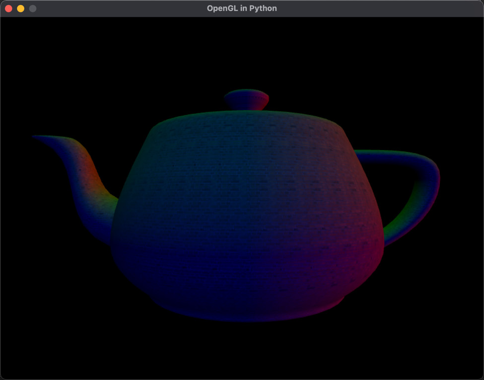
Figure 18.4: The teapot, colored with normal values and textured with a brick pattern
In this exercise, we loaded in a texture and set up UV values for a model. At this point, you know how to use any OBJ model file, along with its texture, in your projects.
Receiving shader compilation errors in Windows
While working with both the macOS and Windows platforms to create this code, I noticed that macOS is a little kinder to small issues concerning shader compilation. If you are using Windows, you will get a compilation error with the fragment shader:
#version 330 core
out vec4 frag_color;
in vec3 normal;
in vec2 UV;
uniform sampler2D tex;
void main()
{
frag_color = vec4(1,1,1,1);
frag_color = frag_color * texture(tex, UV);
}
Why? Because the value of in vec3 normal isn’t used inside the main() function. To fix this, you must remove all mentions of normal and its use from both the vertex and fragment shader, as well as the Python script. The easiest thing to do is comment out its use in the vertex shader, like this:
//in vec3 vertex_normal;;
//out vec3 normal;
//normal = mat3(transpose(model_mat)) * vertex_normal;
Comment out its use in the fragment shader, like this:
//in vec3 normal;
Comment out its use in LoadMesh.py, like so:
#vertex_normals.create_variable(material.program_id,
# “vertex_normal”)
Alternatively, you could leave the normal value being used in the frag_color calculation. The only issue is that you will get a multicolored model. However, this will only happen until we discuss diffuse lighting in the Turning on the lights section.
Your turn...
Exercise A: Load in a properly UVed model and texture by using granny.obj and granny.png, which can be downloaded from GitHub. Modify the fragment shader and remove the normals as colors, and move and reorient the model to make it appear as follows:
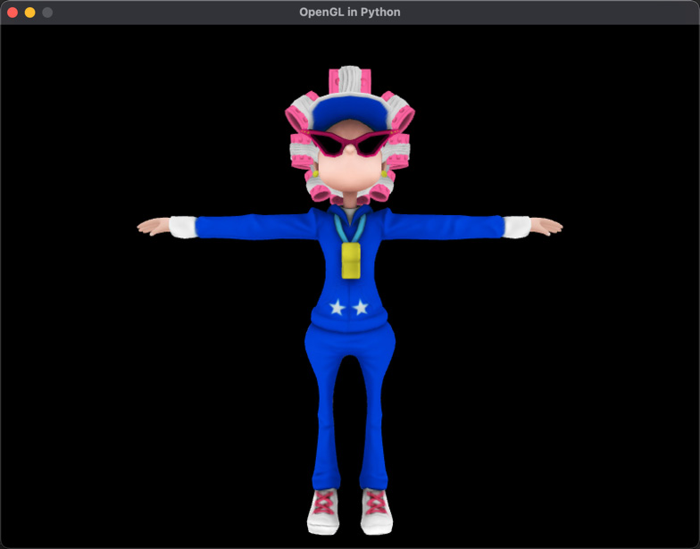
Figure 18.5: A textured model
In this section, we’ve covered using the UVs of a model to place a texture onto that model using shader code. This is the first step in coloring a model and calculating the pixel color using the associated color in the texture file. The second step is to consider how lights in the environment affect the pixel color.
Turning on the lights
When it comes to lighting in shaders, there’s a lot of hands-on mathematics. No longer can we rely on nice, neat OpenGL function calls in our main code. Instead, we must calculate the color of a pixel and consider the lighting in the fragment shader.
In the previous section, when you completed the exercise and loaded the granny model with the texture, it was unlit. It displayed the colors as they appear in the PNG texture file. To include lighting effects, we must determine how the light will influence the original color of the pixel taken from the texture. Over the years, a gradual improvement has been made to lighting models, which is evident if you take a look at the quality of computer graphics from 20 years ago up until now.
In this section, we will examine some popular lighting models and apply the mathematics to our fragment shader to light up the model.
Ambient lighting
Ambient lighting is lighting in a scene that has no apparent source. It is modeled on light that is coming from somewhere but has been scattered and bounced around the environment to provide illumination from everywhere. Think of a very cloudy day. There are no shadows but you can still see objects. The Sun’s light is scattered so much through the clouds that an equal amount of light hits all surfaces.
Ambient lighting is used in computer graphics to illuminate an entire scene. The calculations are straightforward, as you are about to discover.
Let’s do it…
In this exercise, we will calculate and use ambient light in our fragment shader:
- Create a new fragment shader in your project called lighting.vs. Add the following code:
#version 330 core
out vec4 frag_color;
in vec3 normal;
in vec2 UV;
uniform sampler2D tex;
void main()
{vec4 lightColor = vec4(0.5, 0.5, 0.5, 1);float attenuation = 1;vec4 ambient = lightColor * attenuation;frag_color = texture(tex, UV) * ambient;}
Here, an ambient light color of mid-gray is being set. The attenuation is the brightness of the light. To apply ambient light to the pixel color taken from the texture, it is simply multiplied.
- In ShaderTeapot.py (which you may rename ShaderGranny.py if it makes more sense), modify the line of code that loads in the shaders so that it replaces the previous fragment shader:
mat = Material(“shaders/texturedvert.vs”,
“shaders/lighting.vs”)
Running this will result in a dull lit version of the model. You can also change the values of lightColor and attenuation for differing results, as shown in Figure 18.6:
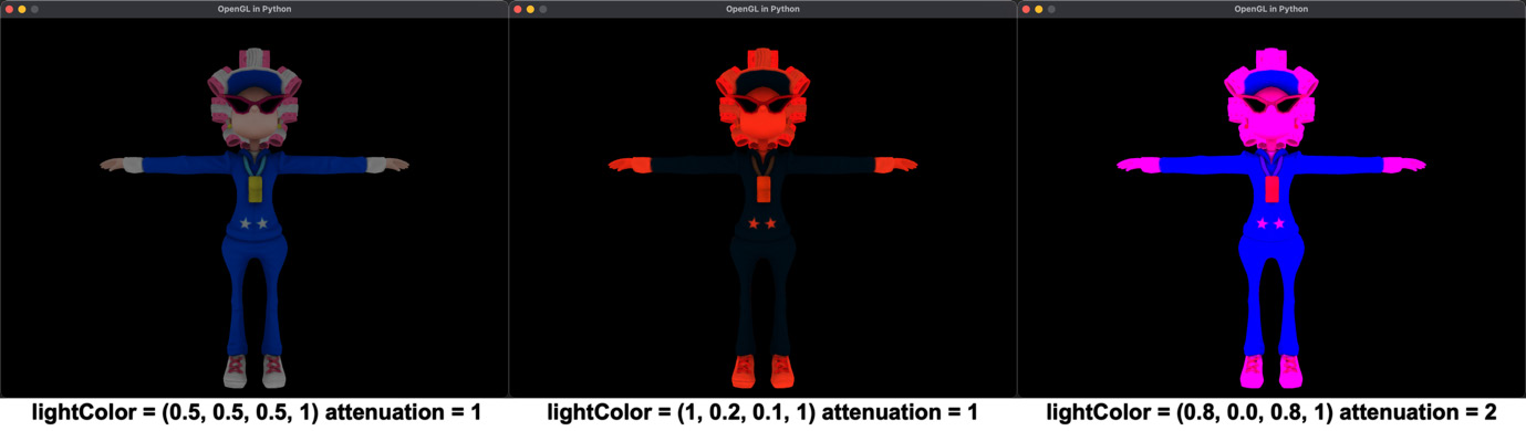
Figure 18.6: Ambient lighting effects
As ambient light does not consider the direction of the light source, there is no apparent shadowing on the object. Ambient light alone can cause a 3D model to lose its depth. This is evident in the right-most image of Figure 18.6, where the pink light has made the image look flat and devoid of any 3D shadowing. The simplest of the lighting models that considers the direction of the light source is the diffuse model.
Diffuse lighting
Diffuse lighting is the simplest form of lighting and is calculated using the normal vector (N) of the surface and the vector representing the direction of the light source (L), as shown in Figure 18.7:
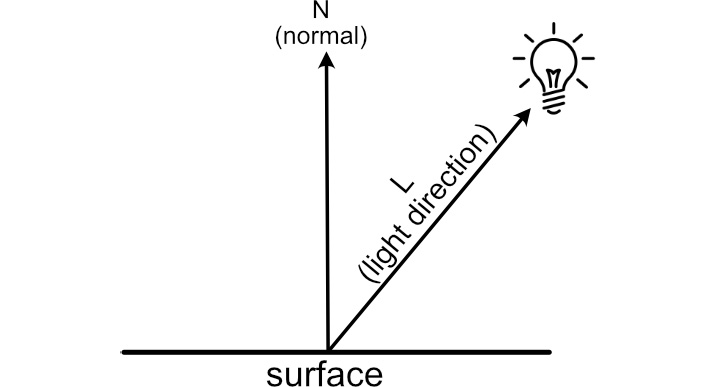
Figure 18.7: Diffuse lighting
In Chapter 9, Practicing Vector Essentials, we learned that we can find the angle between two vectors using the dot product operation. The light will be most intense when it is directly above the surface and the normal and light direction vectors are parallel. The light will not be reflected from the surface if it is orthogonal to the surface or below it. The dot product returns 1 when N and L are parallel, 0 when they are orthogonal, and values less than 0 when L is on the opposite side of the surface to N. The diffuse model states that the higher the value of the dot product, the brighter the surface will appear. Mathematically, we calculate this light intensity (I) as follows:
![]()
We will now use this in the fragment shader.
Let’s do it…
In this exercise, we will modify the fragment shader so that it uses the diffuse lighting model:
- In lighting.vs, modify the main() function in the code like so:
void main()
{vec3 lightDir = vec3(-10,0,5);vec4 lightColor = vec4(1, 1, 1, 1);float NdotL = dot(normalize(normal),normalize(lightDir));float attenuation = 1;vec4 diffuse = lightColor * (NdotL * attenuation);frag_color = texture(tex, UV) * diffuse;}
Notice that a light direction has been added. This is the vector to the light source. At this point in the rendering process, you must consider that the fragment shader is working in screen space, so (0, 0, 0) is the center of the render window. The x coordinates are positive in the right direction, the y coordinates are positive in the up direction, and the z coordinates are negative going into the screen. This would place a light at 5 in the z coordinate, behind the viewer.

Figure 18.8: Diffuse lighting
Diffuse shading injects more depth and shadowing into a scene as it considers the direction of the light source. However, the diffuse lighting model can be improved upon by including the direction for the viewer. This is calculated in the Phong model.
Phong
The Phong lighting model adds specular highlights to a 3D object through the observation that an object has more gloss, shininess, or greater light reflectance based on not only the normal and light direction but also the direction of the viewer, as shown in Figure 18.9:
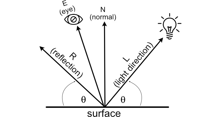
Figure 18.9: Phong lighting
When light hits a surface, it reflects off that surface at the same angle in the opposite direction. This is called the reflection vector. If the eye of the viewer were at the same angle as the reflection vector, they would experience the greatest amount of shininess.
The Phong model expands on the diffuse model by calculating the intensity of light using two factors – diffuse and specular. The diffuse component is calculated as it was previously; the specular component is defined as follows:
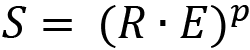
The p variable is called the specular power. The greater the value of p, the more intense the specular highlights. The best way to experience Phong is by working it into our project.
Let’s do it…
In this exercise, we will modify the lighting shader so that it includes specular highlights by implementing the Phong lighting model:
- Modify the code in texturedvert.vs, like so:
#version 330 core
..
uniform mat4 view_mat;
out vec3 normal;
out vec2 UV;
out vec3 view;
void main()
{gl_Position = projection_mat *inverse(transpose(view_mat)) *transpose(model_mat) *vec4(position, 1);UV = vertex_uv;normal = mat3(transpose(model_mat)) *vertex_normal;view = mat3(transpose(model_mat)) * position;}
Here, in the vertex shader, we are adding the view position of the vertex as it is required by the Phong model to calculate the view direction. This is calculated in world space as both the camera and model possess coordinates there.
- Now, we must update lighting.vs so that we can calculate the Phong model:
#version 330 core
out vec4 frag_color;
in vec3 normal;
in vec2 UV;
in vec3 view;
uniform sampler2D tex;
void main()
{float specularPower = 2;vec3 lightDir = normalize(vec3(-10,0,5));vec3 eyeDir = normalize(-view);vec3 norm = normalize(normal);vec3 reflection =normalize(-reflect(lightDir,norm));vec4 lightColor = vec4(1, 1, 1, 1);//diffusefloat NdotL = dot(norm, lightDir);float attenuation = 1;vec4 diffuse = lightColor * (NdotL * attenuation);//specularvec4 specular = lightColor *pow( dot(reflection, eyeDir),specularPower);frag_color =texture(tex, UV) + diffuse + specular;}
The majority of this code has been updated to move the normalization of all vectors to the top of the main section. Note that when working with vectors in shaders, it is best to normalize them. This is because most mathematical functions that use them assume they are normalized, and if the same vector is used multiple times, then it’s more efficient to normalize them just once.
The diffuse and specular components are calculated in separate sections. Diffuse remains as it did previously. For specular, the reflection vector and direction to the viewer (eye) are required, so they are calculated. Shader language provides us with a handy reflect() function to perform the reflection. The direction to the eye from the fragment is calculated using eyeDir = eyePosition – view. However, when in the fragment shader, the eye position is (0, 0, 0) as we are in camera (eye) space. Hence, this calculation can be performed with -view.
After the specular component has been calculated, the final fragment color is devised using the pixel color from the texture and the addition of the diffuse and specular components.
- Run your project now; you’ll find a model with diffuse and shiny specular highlights, as shown in Figure 18.10:
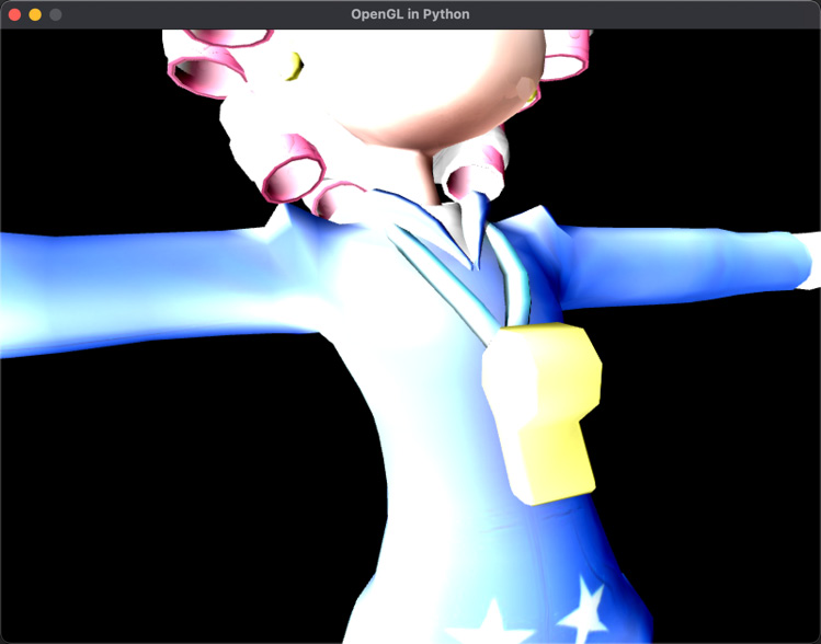
Figure 18.10: Granny light with the Phong model
In this exercise, we learned how to extend the diffuse lighting model so that it uses specular highlights. You can also add the ambient calculations here if you desire. Don’t be afraid to experiment with the colors and intensities – you may just invent an entirely new shading model.
GLSL shading functions
There are many built-in mathematical functions in shader languages, such as the pow() and reflect() methods we’ve just used. As you research other shader code, you’ll come across more of these functions. There are plenty of references to help you understand how each one is used. However, you can get started at https://shaderific.com/glsl/common_functions.html to gain an understanding of the scope of these methods.
In this section, we examined the basics of lighting a model using shaders by exploring the use of ambient, diffuse, and specular lighting. The concepts and extrapolated mathematics are deceptively simple and yet highly effective.
Summary
In this chapter, we changed over the functionality of our project, which was using older OpenGL methods, and replaced the rendering functions with our own vertex and fragment shaders. The shader code we write gets compiled into a program for the graphics processor. You will now have an understanding of how an external script or program written in Python interacts with the shader program. The majority of graphics and games programs are interactive, so being able to process transformations, projections, and camera movements in one program, and send commands to the graphics card for rendering, is a necessary skill for any graphics programmer.
The lighting models we examined here were first created by computer scientists to light scenes with 3D models to create more believable results. Though they are effective and still used today, they don’t quite address the physical nature of the way light interacts in real life.
Nowadays, the more common way to light a scene is with physically based rendering (PBR). This certainly doesn’t do away with ambient, diffuse, and specular lighting, but rather builds upon it by considering the nature of light and how it reacts to different surfaces as it gets absorbed and reflected. In the next and final chapter of this book, we will discuss the mathematics of PBR and build a set of vertex and fragment shaders in GLSL that you can use in your projects.
Answers
Exercise A:
The code only differs from loading the teapot since it loads the granny model:
quat_granny = Object(“Granny”)
quat_granny.add_component(Transform())
mat = Material(“shaders/texturedvert.vs”,
               “shaders/texturedfrag.vs”)
quat_granny.add_component(LoadMesh(quat_granny.vao_ref,
    mat,GL_TRIANGLES, “models/granny.obj”,
    “images/granny.png”))
quat_granny.add_component(mat)
quat_trans: Transform =
    quat_granny.get_component(Transform)
quat_trans.update_position(pygame.Vector3(0, -100, -200))
In the fragment shader, remove the normal from the setup of frag_color (if you aren’t on Windows and haven’t commented out all the error-producing code), like this:
frag_color = vec4(1,1,1,1)