19
Rendering Visual Realism Like a Pro
As graphics cards and the resolution of computer displays have improved over time, audiences have expected better quality rendering in animated movies, games, and other computer graphics-based media. By examining the way that objects in the real world get their color, computer scientists have been able to improve upon similar models of Lambert and Phong. Today, most 3D engines aimed at producing visual realism apply a shading technique called physically based rendering (PBR).
In this chapter, we will investigate the theory behind this technique and then put it into practice in our Pygame/OpenGL project. To this end, we will be discussing the following topics in this chapter:
- Following where light bounces
- Applying the Inverse Square Law
- Calculating Bidirectional Reflectance
- Putting it all together
By the end of this chapter, you will have a project that uses Python and OpenGL to render objects using PBR and understand all the components that are combined to create the final effect. This knowledge will assist you in moving forward with your independent learning of graphics to improve your own projects and also help identify improvements for others.
Technical requirements
The solution files containing the code in this chapter can be found on GitHub at https://github.com/PacktPublishing/Mathematics-for-Game-Programming-and-Computer-Graphics/tree/main/Chapter19 in the Chapter19 folder.
Following where light bounces
PBR is based on the actual physics of light rather than the other relatively simple lighting model of Lambert, examined in Chapter 5, Let’s Light It Up! PBR is a concept rather than a specific algorithm and can be achieved using a variety of mathematical models. To understand how PBR works, we need to understand some key fundamentals about the visual way light works.
Light is a ray we can represent with vectors relative to the normal of the surface being hit, as shown in Figure 19.1:
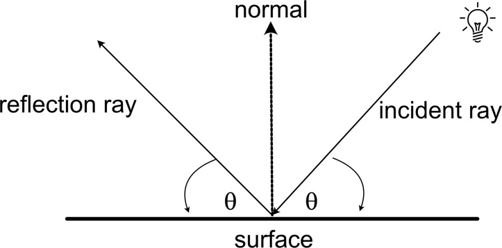
Figure 19.1: An incident and reflection ray
The light coming in from the source is called the incident ray and the light being reflected from the surface is called the reflection ray. According to the law of reflection, the angle of incidence is equal to the angle of reflection. Both rays travel in a straight line, and whether the strength of the incoming ray is the same as the reflected ray depends on what happens at the point of collision.
We also need to consider how light behaves when it passes from one medium to another. A medium can be anything, from air to metal to wood or water. Whenever the density of the medium changes, the light ray will be affected at the point of contact, depending on the change in density from one medium to another. The amount that light is refracted is called the refractive index. Some of the light will be reflected and some will pass into the medium. At the point of collision, the ray is bent in another direction. This is called refraction. We experience the refraction of light when looking at objects placed in water where they undergo a visual separation of themselves above the water and more dramatically when pure white light passes through a prism that splits into eight separate color components, as illustrated in Figure 19.2:
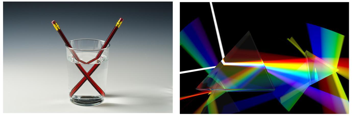
Figure 19.2: Light refraction examples
PBR enforces the principle of energy conservation, which states that the total amount of light after hitting a surface remains the same. Some is reflected, some is refracted, and some is absorbed.
What happens at the point of contact influences how we will see things. When light hits a mirror or highly metallic surface, almost all the light is reflected, none is refracted, and very little is absorbed. Therefore, the reflected light is almost as bright and the same color as the incoming light. Some metals absorb light at different wavelengths. For example, gold absorbs mostly blue light and reflects yellow, and hence it appears yellow.
Smooth polished objects appear shinier because of the way they reflect light. However, if you could examine such a surface on a micro level, you would see all the imperfections, as shown in Figure 19.3. This doesn’t go unnoticed by a ray of light. These imperfections create many differing normals on the surface being hit, and therefore, the reflected ray is scattered. This dulls the appearance of the reflection. In addition, a rough surface can also make a metallic surface look less shiny because of the obvious imperfections scattering the rays, as illustrated by the brass plates in Figure 19.3:
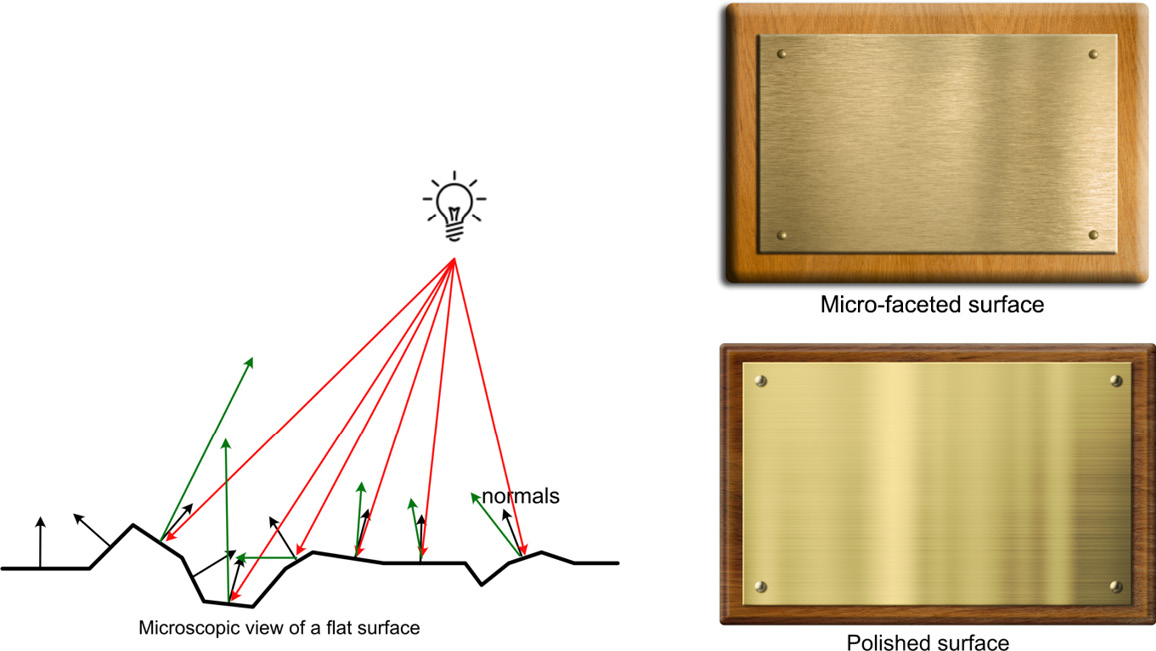
Figure 19.3: A close-up view of a surface with micro-facets and normals and the different reflections of metal surfaces
Light rays not only bounce around an environment; their strength also diminishes over distance. This is another important factor to consider when attempting to render visual realism. We will now examine the mathematics that we can apply to calculate this effect.
Applying the Inverse Square Law
The way that the strength of light gets weaker with distance from the light source is described by the inverse square law. It states that the light intensity gets inversely weaker based on the square of the distance the viewer is away from the light source. Mathematically, we represent it like this:

Just how quickly the light strength falls off with distance will depend on the medium through which the light is traveling. We can calculate the strength of light at a certain distance in the same medium if we know its strength for a previously measured distance. For example, if the light intensity is 10 at a distance of 100 meters from the source, we can calculate the strength that this same light will be at 125 meters, using proportions like this:

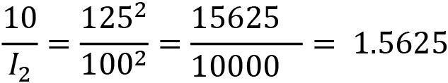
![]()
This answer makes sense if we think about it as the same light at a further distance being less bright.
The strength of the light being emitted from the light source, as we discussed in Chapter 18, Customizing the Render Pipeline, is called attenuation, and how much it lights up a surface is known as the radiance.
To produce a radiance factor for numerous lights in a shader, we add the radiance of each light after determining the value of radiance, given the attenuation and distance that the light source is from the vertex or fragment. Here’s some pseudo code that explains the calculations:
vec3 total_radiance = 0;
for(int i = 0; i < NUM_LIGHTS; ++i) //each light
{
    float distance    = length(light_data[i].position –
                               vertex_pos);
    float attenuation = light_data[i].attenuation /
                                   (distance * distance);
    vec3 radiance     = light_data[i].color * attenuation;
    total_radiance += radiance;
}
We will put this code into our own shader soon. However, before we do, we need to consider the other influencing factors in building a PBR shader, most of which are defined by customizable reflectance functions.
Calculating Bidirectional Reflectance
Besides ordinary reflectance and scattering, PBR also integrates a bidirectional reflectance distribution function (BRDF), which considers how a specular reflection will fall off or how fuzzy it appears around the edges. It is a function that considers the four factors of the incident ray, the vector to the viewer, the surface normal, and radiance (how well the surface reflects light). In fact, the Lambert (diffuse) and Phong (specular) models we considered in Chapter 18, Customizing the Render Pipeline, are examples of BRDFs. The BRDF for Phong, which calculates specular lighting that can be added to the diffuse of Lambert for a final effect, can be stated as the following:
![]()
In this formula, R is the vector of reflection of the incoming light, E is the vector from the point of contact to the viewer’s eye, and p is the specular power. All vectors involved in calculating reflections are shown in Figure 19.4:
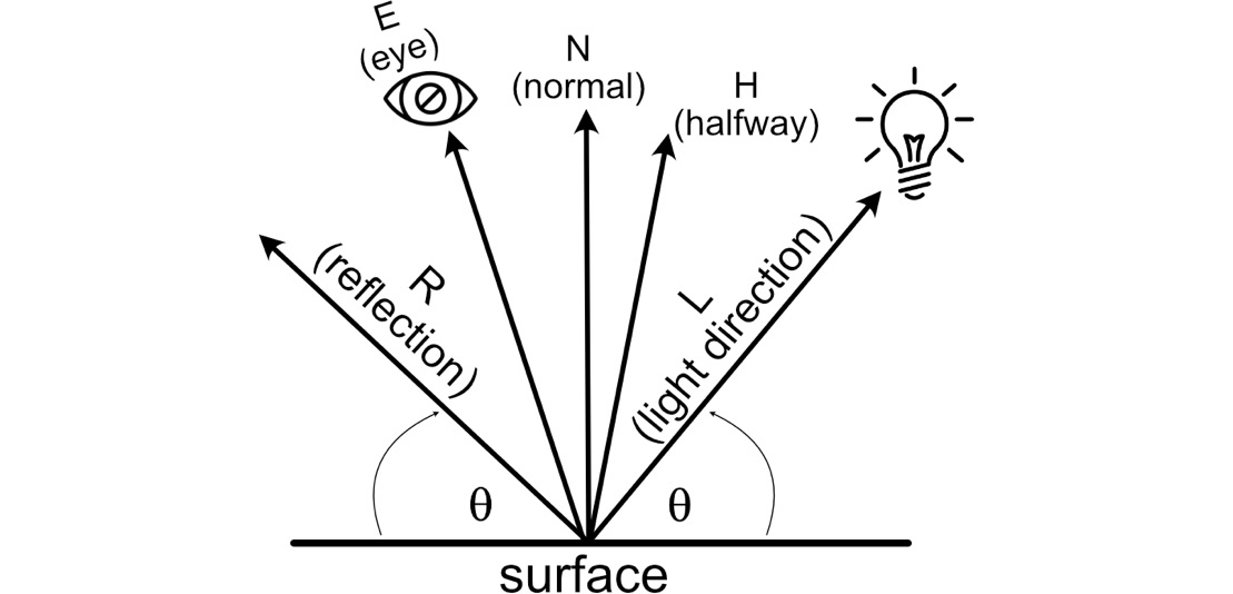
Figure 19.4: Vectors used in reflectance models
However, since the first use of Lambert, Phong, and other early reflectance models in computer graphics in the early 1970s, many updated models have been devised that consider anisotropic reflection, the Fresnel effect, and micro-facets.
One such model is the Cook-Torrance Model (https://graphics.pixar.com/library/ReflectanceModel/), which is a specular-only model considering the shininess of objects while integrating factors for micro-faceting. It takes the following form:
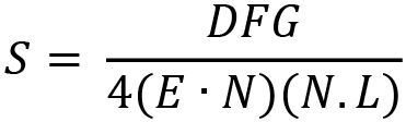
The values of D, F, and G are the functions for a distribution function, the Fresnel effect, and geometric attenuation respectively. Each returns a further lighting calculation that is integrated into the final result. Basically, these three functions are plug and play – that is, there are multiple ways of calculating each one. Specifically, we will examine the work of computer graphics scientists Beckman (https://aip.scitation.org/doi/10.1063/1.325037), Smith (https://ieeexplore.ieee.org/abstract/document/1138991), and Schlick (https://citeseerx.ist.psu.edu/viewdoc/download?doi=10.1.1.50.2297&rep=rep1&type=pdf). We will take a look at some of these now.
Distribution functions
There are numerous distribution functions that can be used in the Cook-Torrance model. We will examine two of the most commonly used – Beckmann and GGX.
Beckmann distribution is a model used in PBR to calculate reflectance factors for micro-facets. The distribution formula results in the D value, which indicates how rough or smooth a surface is. It’s described by this equation:
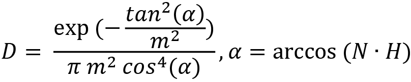
In this equation, the value of m2 is the root mean square of the slopes of all the micro-facets. This is the average of all the gradients of the microfacet edges, each squared, and then added together. This provides the formulae with a roughness value between 0 and 1, where 0 indicates the surface is super smooth and 1 that it is extremely rough. If you were to manually measure all the slopes of the surface’s micro-facets, squaring them, and then calculate the mean, it would be an arduous if not impossible task. Therefore, a distribution function provides us with a guesstimate of how smooth a surface is using a single roughness value.
The value of the H vector is a vector sitting halfway between the light direction and eye direction vectors shown in Figure 19.4. It first originated in the Blinn-Phong reflectance model, which we’ve not had the space to investigate herein, although if you are interested, you should follow it up here: learnopengl.com/Advanced-Lighting/Advanced-Lighting.
A simpler and less processor-heavy distribution function is GGX, introduced here: www.cs.cornell.edu/~srm/publications/EGSR07-btdf.pdf. It provides a better match to real-world reflections than Beckmann, and provides micro-faceting calculations on a number of surfaces. It is defined as the following:

The GLSL implementation of this distribution function is as follows:
float GGX(float NoH, float roughness)
{
    float a = roughness*roughness;
    float a2 = a*a;
    float NoH2 = NoH*NoH;
    float numerator = a2;
    float denominator = (NoH2 * (a2 - 1.0) + 1.0);
    denominator = PI * denominator * denominator;
    return numerator / denominator;
}
In this code, you will find each element of the preceding equation for GGX broken down into its components. Given the dot product between the normal and halfway vector and a value for how rough the surface is, the function will return the value of D, the roughness distribution value that we can later use in calculating the Cook-Torrance BRDF.
The Fresnel effect
The Fresnel effect is the observation that the amount of reflection is highest when the viewing angle with respect to the surface normal is large. This is easily observed when examining a pool of water. If you look straight down into the water, you’ll be able to see the bottom. However, when you look at it from a sharp angle, close to the water surface, it will be highly reflective, as illustrated in the photos in Figure 19.5:
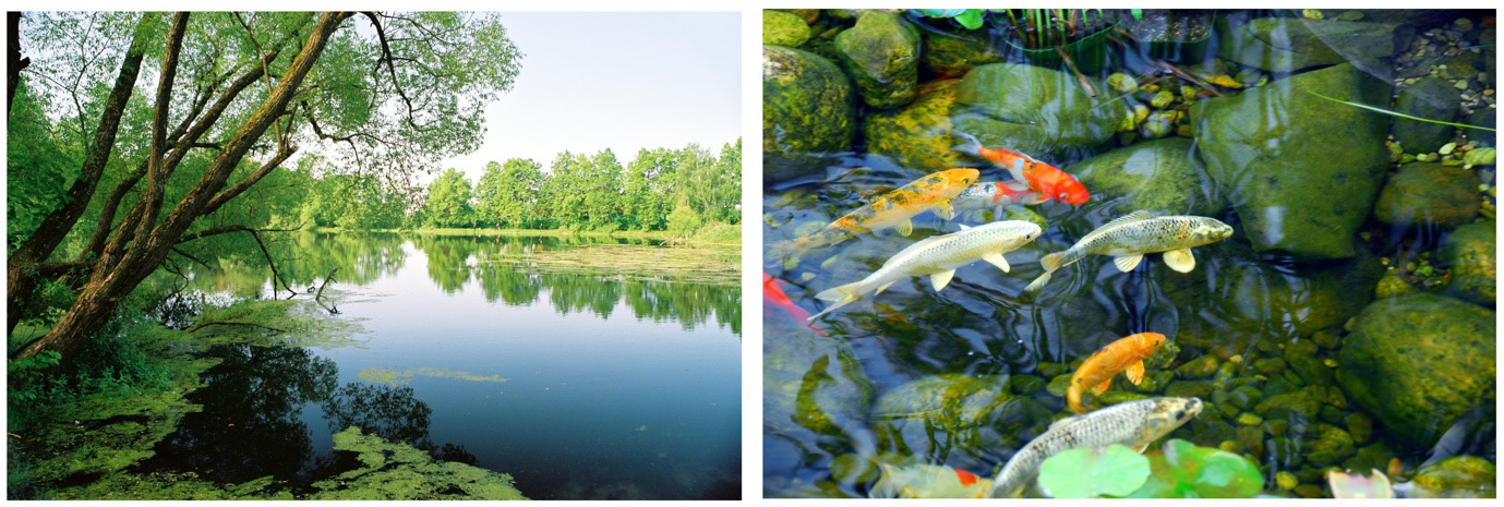
Figure 19.5: Looking into water from different angles
When looking across the lake, the sky and the trees beyond are clearly reflected on the water’s surface. However, when looking down into the water at a higher angle, there’s far less reflection and it is easier to see the bottom.
Looking across a surface almost in parallel with that surface is called a grazing angle because you’re almost grazing the surface. For a smooth surface, such as water or even smooth plastic, the reflectance tends to be very close to 100%. For rough surfaces, it is much less but reflection is still possible.
An inexpensive approximation for calculating the Fresnel term was devised by researcher Christophe Schlick and takes the optimized form:

The metallic parameter in this formula is a value between 0 and 1 that describes how close a surface is to replicating metal. For a metallic surface, the Fresnel effect is greater, as metals reflect light more readily.
The GLSL implementation of this Fresnel approximation function is as follows:
vec3 Fresnel(float HoV, vec3 metalness)
{
    return metalness + (1.0 - metalness) *
                   pow(clamp(1.0 - HoV, 0.0, 1.0), 5.0);
}
The use of the clamp function here is to ensure (1.0 – HoV) does not go outside the range of 0 and 1.
Geometric attentuation factor
The geometric attenuation factor is a value that describes the self-shadowing and masking on a surface due to micro-facets. Its equation is in the following form:

And the GS function is defined as the following:
It returns a single float value that is multiplied by the distribution function and Fresnel equation results to add even more visual realism to a surface.
The GLSL implementation of Smith’s approximation function with Schlick’s optimization, according to the preceding equations, is the following:
float GASchlick(float NoV, float roughness)
{
    float r = (roughness + 1.0);
    float k = (r*r) / 8.0;
    float numerator   = NoV;
    float denominator = NoV * (1.0 - k) + k;
    return numerator / denominator;
}
float GASmith(float NoV, float NoL, float roughness)
{
    float gas2  = GASchlick(NoV, roughness);
    float gas1  = GASchlick(NoL, roughness);
    return gas1 * gas2;
}
In this code, you will find the preceding formulae for geometric attenuation broken down into their elements to calculate a value for G.
Further references
For more functions that can be used with BRDF and further mathematical explanations, please see these excellent references:
https://google.github.io/filament/Filament.html
https://learnopengl.com/PBR/Theory
In this section, we’ve covered the primary mathematics required to implement a PBR shader with particular emphasis on the BRDF. Along with direct light information, coloring, and ambient lighting, we can now implement a full PBR shader into our project.
Putting it all together
PBR lighting models are used in many game engines, including Unity and Unreal. Walt Disney Pictures and Pixar also use PBR to light their 3D animations, and in fact, the models you’ve learned about herein are used in their graphics tools.
What distinguishes the BRDF used by PBR is that it allows for the use of parameters. These parameters allow you to customize the look of the shader and define the surface qualities of objects, using albedo for the diffuse color and values for metallicness, roughness, and ambient occlusion (AO).
Now, it’s time to put all this theory into practice, so we can see it at work in our Python/OpenGL project.
Let’s do it…
In this exercise, we will rework the project to pass the settings for albedo, metallic, roughness, and ambient occlusion through to the shaders, in addition to adding multiple lights:
- Make a copy of the Chapter_18 folder and rename it Chapter_19.
- You will need a copy of the sphere.obj model file available in GitHub. Make sure you add it to the models folder of Chapter_19 for your project.
- Make a copy of ShaderTeapot.py or the file you copied from this and displayed the Granny model in Chapter 18, Customizing the Render Pipeline. Call this copied file PBR.py. Make the following changes:
..
from Settings import *
from Light import *
pygame.init()
..
objects_3d = []
camera = Camera(60, (screen_width / screen_height),
0.01, 10000.0)for x in range(10):
for y in range(10):sphere = Object(“Sphere”)sphere.add_component(Transform())mat = Material(“shaders/pbrvert.vs”,“shaders/pbrfrag.vs”)sphere.add_component(LoadMesh(sphere.vao_ref, mat,GL_TRIANGLES,“models/sphere.obj”))sphere_mesh: LoadMesh =sphere.get_component(LoadMesh)sphere_mesh.set_properties(pygame.Vector3(1, 0, 1),x/10.0, x/10.0, y/10.0)sphere.add_component(mat)sphere_trans: Transform =sphere.get_component(Transform)sphere_trans.update_position(pygame.Vector3(x*20, y*20, -20))objects_3d.append(sphere)
Here, we are adding nested loops that range the values of x and y from 0 through to 10. As the x and y values change, they are used to position the spheres and also to set the properties. The set_properties() method we are yet to add to the LoadMesh() class will allow you to set the albedo, metallic, roughness, and ambient occlusion values that each sphere will use as a customized setting sent to the shader.
This code includes a newly imported file that we are yet to write (Light.py); however, it will define the lights you are adding here:
lights = []
lights.append(Light(pygame.Vector3(0, 100, 200),
                    pygame.Vector3(0, 1, 1), 5, 0))
lights.append(Light(pygame.Vector3(0, 50, 200),
                    pygame.Vector3(1, 0, 1), 2, 1))
lights.append(Light(pygame.Vector3(100, 0, 200),
                    pygame.Vector3(1, 1, 0), 5, 2))
..
pygame.mouse.set_visible(False)
while not done:
    ..
    glClear(GL_COLOR_BUFFER_BIT | GL_DEPTH_BUFFER_BIT)
    camera.update()
    for o in objects_3d:
        o.update(camera, lights, events)
..
You can see the lights are placed into an array, called lights, after a set of spheres is created from the newly added sphere.obj model.
The parameters passed to the creation of the lights specify their location in the world, their color, their attenuation, and the position at which they appear in the array.
- Create a new Python script called Light.py and add the following:
from Transform import *
class Light:
def __init__(self, position=pygame.Vector3(0, 0,0),color=pygame.Vector3(1, 1, 1),atten=0, light_number=0):self.position = positionself.atten = attenself.color = colorself.light_variable =“light_data[“ + str(light_number) +“].position”self.atten_variable = “light_data[“ +str(light_number) + “].attenuation”self.color_variable = “light_data[“ +str(light_number) + “].color”
The position and color for each light are set as Vector3. In the initialization, three variable strings for each light are also defined. They specify what the light is called in the shader code. It is essential they are spelled here as they are in the shader. For example, if the light has a light_number of 2, then the self.light_variable string will contain light_data[2].position. You’ll see where this goes in the shader code in step 10.
- Because the lights are objects that apply to each and every object in the 3D environment, they are dealt with like the camera. Open Object.py and modify the code thus:
from LoadMesh import *
..
from Light import *
class Object:
def __init__(self, obj_name):..def add_component(self, component):..)def get_component(self, class_type):..def update(self, camera: Camera,lights: Light([]), events = None):self.material.use()for c in self.components:if isinstance(c, Transform):..transformation.load()for l in lights:light_pos = Uniform(“vec3”,l.position)light_pos.find_variable(self.material.program_id,l.light_variable)light_pos.load()light_atten = Uniform(“float”,l.atten)light_atten.find_variable(self.material.program_id,l.atten_variable)light_atten.load()color = Uniform(“vec3”, l.color)color.find_variable(self.material.program_id,l.color_variable)color.load()elif isinstance(c, LoadMesh):c.draw()
In this code, lights are passed to the update() function as an array. This array is looped over and the uniform variables in the shader for the light’s position, color, and attenuation are passed through.
- LoadMesh.py also needs a small modification, thus:
class LoadMesh(Mesh3D):
def __init__(self, vao_ref, material, draw_type,model_filename, texture_file=””,back_face_cull=False):..
#Comment out v_uvs as they aren’t needed for#the shader and will cause Windows errors#v_uvs = GraphicsData(“vec2”, self.uv_vals)#v_uvs.create_variable(# self.material.program_id,# “vertex_uv”)self.albedo = Noneself.metallic = Noneself.roughness = Noneself.ao = None#Comment out these next lines or remove them.#if texture_file is not None:#self.image = Texture(texture_file)#self.texture = Uniform(“sampler2D”,#[self.image.texture_id,# 1])def format_vertices(self, coordinates, triangles):..def set_properties(self, albedo, metallic,roughness, ao):self.albedo = Uniform(“vec3”, albedo)self.metallic = Uniform(“float”, metallic)self.roughness = Uniform(“float”, roughness)self.ao = Uniform(“float”, ao)def draw(self):self.albedo.find_variable(self.material.program_id,“albedo”)self.albedo.load()self.metallic.find_variable(self.material.program_id,“metallic”)self.metallic.load()self.roughness.find_variable(self.material.program_id,“roughness”)self.roughness.load()self.ao.find_variable(self.material.program_id, “ao”)self.ao.load()glBindVertexArray(self.vao_ref)glDrawArrays(self.draw_type, 0,len(self.coordinates))..
The new LoadMesh.py script passes through the values for the albedo, metallic, roughness, and AO that are set when the spheres are created in PBR.py through the shader. Most of these values are floats and uniforms; therefore, our Uniform.py class needs to deal with float values. The albedo is a Vector3 struct that represents the color of a pixel, and metallicness, roughness, and ambient occlusion are values between 0 and 1, representing either all of that property or none. A value of 1 for metallic would specify that the object to be rendered should be treated like a pure metal, such as gold. Roughness, when set to smooth, will give a very mirror-like finish with no micro-facets. The value of AO specifies how much of any pixel is in shadow.
- Open Uniform.py and add the following code:
def load(self):
if self.data_type == “vec3”:glUniform3f(self.variable_id, self.data[0],self.data[1], self.data[2])elif self.data_type == “float”:glUniform1f(self.variable_id, self.data)elif self.data_type == “mat4”:glUniformMatrix4fv(self.variable_id, 1,GL_TRUE, self.data) - Now, it’s time to write the shader code. Create two files in the shader folder – one called pbrvert.vs and the other called pbrfrag.vs.
- To pbrvert.vs, add the following:
#version 330 core
in vec3 position;
in vec3 vertex_normal;
uniform mat4 projection_mat;
uniform mat4 model_mat;
uniform mat4 view_mat;
out vec3 normal;
out vec3 world_pos;
out vec3 cam_pos;
void main()
{gl_Position = projection_mat * transpose(view_mat)* transpose(model_mat) *vec4(position, 1);normal = mat3(transpose(model_mat)) *vertex_normal;world_pos = (transpose(model_mat) *vec4(position, 1)).rgb;cam_pos = vec3(inverse(transpose(model_mat)) *vec4(view_mat[3][0],view_mat[3][1],view_mat[3][2],1));}
This is very similar to vertex shaders we’ve written in the past; however, we are now passing through the world_pos (world position) of the vertex as well as the cam_pos (camera position). These will be required to calculate and deal with real-world vectors for the eye-viewing direction and lighting calculations.
- To pbrfrag.vs, add the following:
#version 330 core
out vec4 frag_color;
in vec3 world_pos;
in vec3 normal;
in vec3 cam_pos;
// material parameters
uniform vec3 albedo;
uniform float metallic;
uniform float roughness;
uniform float ao;
struct light
{vec3 position;vec3 color;float attenuation;};
#define NUM_LIGHTS 3
uniform light light_data[NUM_LIGHTS];
const float PI = 3.14159265359;
void main()
{vec3 N = normalize(normal);vec3 V = normalize(cam_pos - world_pos);vec3 color = vec3(0,0,0);for(int i = 0; i < NUM_LIGHTS; ++i) //each light{// calculate per-light radiancevec3 L = normalize(light_data[i].position -world_pos);vec3 H = normalize(V + L);float distance =length(light_data[i].position -world_pos);float attenuation = light_data[i].attenuation/(distance * distance);vec3 radiance = light_data[i].color *light_data[i].attenuation;color += radiance;}color *= albedo * roughness * metallic *ao * normal;frag_color = vec4(color, 1.0);}
In this code, we’ve now set up the values of world_pos and cam_pos to be passed from the vertex shader, and also created uniform values to accept albedo, metallic, roughness, and AO values.
Inside the main function, each light is looped over to add up its radiant effect on a fragment using its color, attenuation, and distance from the fragment.
The remainder of the fragment shader does not do anything special but ensures that, at this point, you can press Play and render something, as shown in Figure 19.6:
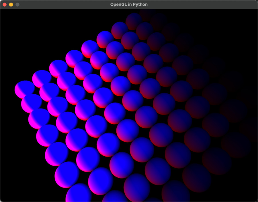
Figure 19.6: A grid of spheres with lighting effects
Note
As, at this point, we have not implemented a PBR shader, if you can’t see anything in the window, try flying around with the camera to see whether you are facing it in the wrong direction.
- It’s time to modify the fragment shader to produce a PBR effect. Open pbrfrag.vs and make these modifications:
#version 330 core
..
#define NUM_LIGHTS 3
uniform light light_data[NUM_LIGHTS];
const float PI = 3.14159265359;
vec3 Fresnel(float HoV, vec3 metalness)
{return metalness + (1.0 - metalness) *pow(clamp(1.0 - HoV, 0.0, 1.0), 5.0);}
float GGX(float NoH, float roughness)
{float a = roughness*roughness;float a2 = a*a;float NoH2 = NoH*NoH;float numerator = a2;float denominator = (NoH2 * (a2 - 1.0) + 1.0);denominator = PI * denominator * denominator;return numerator / denominator;}
float GASchlick(float Ndot, float roughness)
{float r = (roughness + 1.0);float k = (r*r) / 8.0;float numerator = Ndot;float denominator = Ndot * (1.0 - k) + k;return numerator / denominator;}
float GASmith(float NoV, float NoL, float roughness)
{float gas2 = GASchlick(NoV, roughness);float gas1 = GASchlick(NoL, roughness);return gas1 * gas2;}
First, we add the functions for each of the methods required by the Cook-Torrance BDRF. These are the same functions we looked at in the Calculating bidirectional reflectance section.
Next, we modify the main function to use these functions and calculate the BRDF:
void main()
{
    vec3 N = normalize(normal);
    vec3 V = normalize(cam_pos - world_pos);
    vec3 metalness = vec3(0.01);
    metalness = mix(metalness, albedo, metallic);
    // reflectance equation
    vec3 totalRadiance = vec3(0.0);
    for(int i = 0; i < NUM_LIGHTS; ++i) //each light
    {
        ..
        float attenuation = light_data[i].attenuation
                            / (distance * distance);
        vec3 radiance     = light_data[i].color *
                  light_data[i].attenuation;
        // Cook-Torrance BRDF
        float D = GGX(max(dot(N, H), 0.0), roughness);
        float G   = GASmith(max(dot(N, V), 0.0),
                    max(dot(N, L), 0.0), roughness);
        vec3 F    = Fresnel(max(dot(H, V), 0.0),
                            metalness);
        vec3 numerator    = D * G * F;
        float denominator = 4.0 * max(dot(N, V), 0.0)
            * max(dot(N, L), 0.0) + 0.0001;
        vec3 specular     = numerator / denominator;
        // add to total radiance
        float NoL = max(dot(N, L), 0.0);
        totalRadiance += (albedo / PI + specular) *
                          radiance * NoL;
    }
    vec3 ambient = vec3(0.01) * albedo * ao;
    vec3 color = ambient + totalRadiance;
    color = color / (color + vec3(1.0));
    color = pow(color, vec3(1.0/2.2));
    frag_color = vec4(color, 1.0);
}
Here, the BDRF is calculated. The Cook-Torrance formula is for specular reflection only, and therefore, immediately after calculating the specular (for each light), which uses the variables for metallic and roughness, the albedo and AO are also integrated.
Running the project now, you will find a grid of spheres with differing metallic, roughness, and AO values, as shown in Figure 19.7:
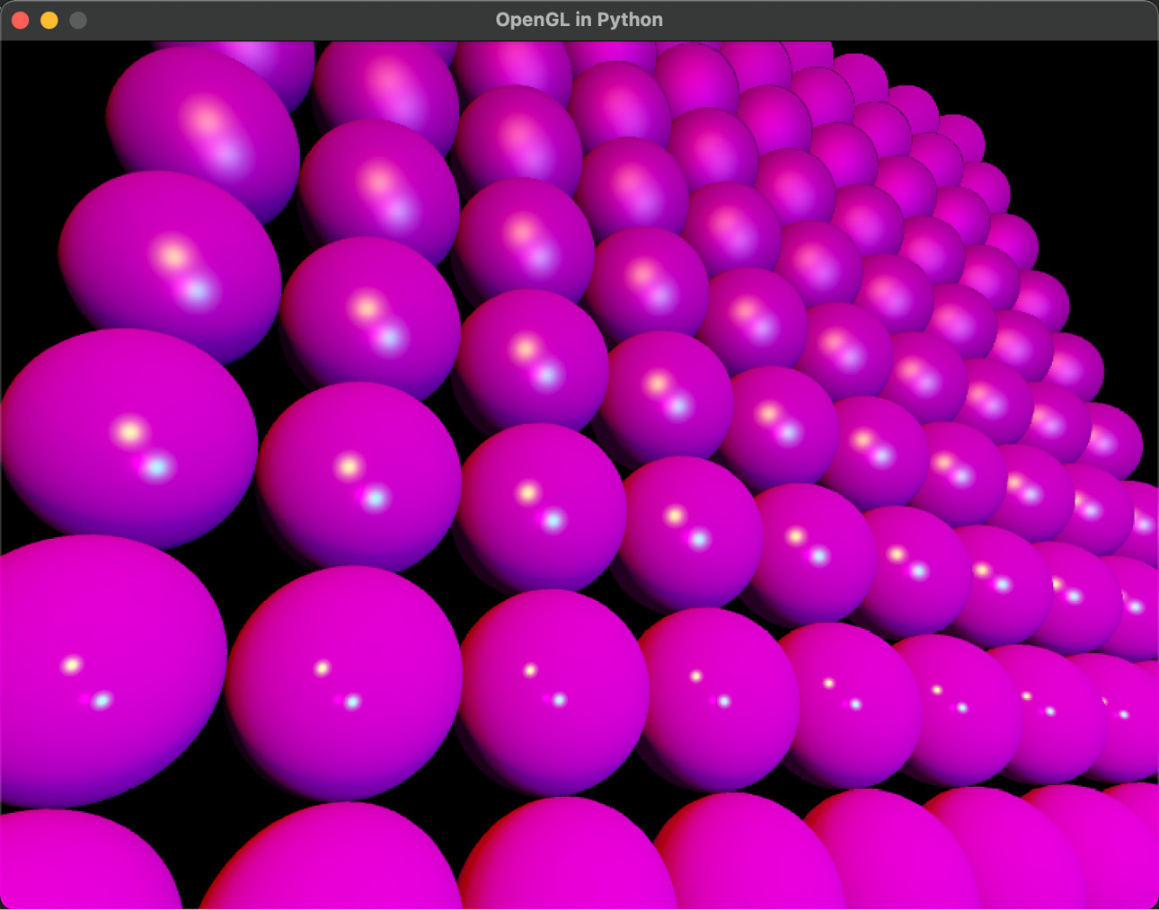
Figure 19.7: PBR of spheres with different parameters
If you’d like to examine the albedo, metallic, roughness, and AO parameter effects on individual spheres, replace the nested for loop in pbr.py to draw just one sphere with differing values, as shown in Figure 19.8:
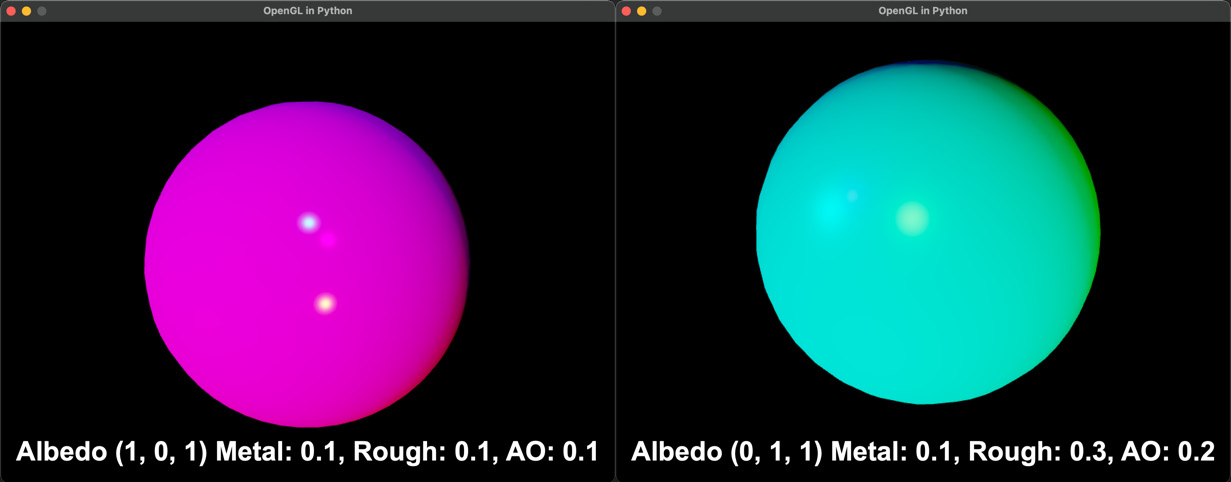
Figure 19.8: Spheres with different PBR treatments
In this exercise, you’ve created the first version of a PBR shader and used it to render spheres with different settings for albedo, metallicness, roughness, and ambient occlusions. As discussed, PBR is an idea for shading and not a fixed algorithm, so feel free to play with the values. I’m certain as you continue to independently investigate more shading techniques and improvements on this basic PBR shader we have created, you will be able to integrate them into your project.
Summary
As you’ve explored in this chapter, there’s a lot of mathematics involved in creating shaders, although the basics still focus on the vectors that explain the direction of a surface with respect to the position of the light and the location of the viewer. With the addition of a few extra PBR parameters of metallicness, roughness, and AO, we are now also able to define how a surface scatters light and use that to improve a final render.
Your Python/OpenGL project is now at the point that you can continue to independently research graphics and shader techniques and experiment with them in the base that you have. You will now have a firm foundation of knowledge in this area that you can apply in the future to games and other applications alike.
The domain of mathematics involved in computer games and graphics is enormous. Unfortunately, books have page limits and authors have limited writing time. To cover everything in this field would require a set of encyclopedic volumes that would have to be updated daily. However, the underlying mathematics doesn’t change. It is my hope that through reading the content herein, you will not only expand your knowledge and skills in this area but also feel confident while going forward in your own independent explorations of the content in this field, and someday add to it.
There’s a never-ending list of books and online tutorials about mathematics in games and graphics to keep you busy for millennia. It’s my expectation that you will read this book and be impassioned to further investigate this field, feeling confident in the skills you’ve obtained herein to dive into the work of others.
Where do you go from here? Well, I can recommend my own tutorials and resources at h3dlearn.com and youtube.com/c/holistic3d, although you might also want to investigate a couple of the texts that first inspired me to enter this field:
- Foley, J. D., Van, F. D., Van Dam, A., Feiner, S. K., & Hughes, J. F. (1996). Computer graphics: principles and practice (Vol. 12110). Addison-Wesley Professional.
- Hill Jr, F. S. (2008). Computer graphics using OpenGL. Pearson Education.
By giving you these older references, I’m pointing out that technology changes but the fundamentals of mathematics remain.
If you are further keen to investigate the use of shaders with Python and OpenGL, there’s an excellent resource with shader code at shadertoy.com, and I have a YouTube series of tutorials that explain how to convert the shaders on this site for use in the code you are now familiar with: https://youtube.com/playlist?list=PLi-ukGVOag_2FRKHY5pakPNf9b9KXaYiD.
Wherever your mathematics, games, and graphics journey takes you from here, all my very best wishes, and I hope you develop the same passion for this field that I have.