
In this recipe, we will show an example of FFT (Fast Fourier Transform) data visualization on a circular layout with some smooth animation.
We will create visualization based on an example FFT analysis using the following steps:
- Include the following necessary header files:
#include "cinder/gl/gl.h"
#include "cinder/audio/Io.h"
#include "cinder/audio/Output.h"
#include "cinder/audio/FftProcessor.h"
#include "cinder/audio/PcmBuffer.h"
- Add the following members to your main application class:
void drawFft();
audio::TrackRef mTrack;
audio::PcmBuffer32fRef mPcmBuffer;
uint16_t bandCount;
float levels[32];
float levelsPts[32];
- Inside the
setupmethod, initialize the members and load the sound file from the assets folder. We are decomposing the signal into 32 frequencies using FFT:bandCount = 32; std::fill(boost::begin(levels), boost::end(levels), 0.f); std::fill(boost::begin(levelsPts), boost::end(levelsPts), 0.f); mTrack = audio::Output::addTrack( audio::load( getAssetPath("music.mp3").c_str() ) ); mTrack->enablePcmBuffering( true ); - Implement the
updatemethod as follows:mPcmBuffer = mTrack->getPcmBuffer(); for( int i = 0; i< ( bandCount ); i++ ) { levels[i] = max(0.f, levels[i] - 1.f ); levelsPts[i] = max(0.f, levelsPts[i] - 0.95f ); } - Implement the
drawmethod as follows:gl::enableAlphaBlending(); gl::clear( Color( 1.0f, 1.0f, 1.0f ) ); gl::color( Color::black() ); gl::pushMatrices(); gl::translate(getWindowCenter()); gl::rotate( getElapsedSeconds() * 10.f ); drawFft(); gl::popMatrices();
- Implement the
drawFftmethod as follows:float centerMargin= 25.0f; if( !mPcmBuffer ) return; std::shared_ptr<float> fftRef = audio::calculateFft( mPcmBuffer->getChannelData( audio::CHANNEL_FRONT_LEFT ), bandCount ); if( !fftRef ) { return; } float *fftBuffer = fftRef.get(); gl::color( Color::black() ); gl::drawSolidCircle(Vec2f::zero(), 5.f); glLineWidth(3.f); float avgLvl= 0.f; for( int i= 0; i<bandCount; i++ ) { Vec2f p = Vec2f(0.f, 500.f); p.rotate( 2.f * M_PI * (i/(float)bandCount) ); float lvl = fftBuffer[i] / bandCount * p.length(); lvl = min(lvl, p.length()); levels[i] = max(levels[i], lvl); levelsPts[i] = max(levelsPts[i], levels[i]); p.limit(1.f + centerMargin + levels[i]); gl::drawLine(p.limited(centerMargin), p); glPointSize(2.f); glBegin(GL_POINTS); gl::vertex(p+p.normalized()*levelsPts[i]); glEnd(); glPointSize(1.f); avgLvl += lvl; } avgLvl /= (float)bandCount; glLineWidth(1.f); gl::color( ColorA(0.f,0.f,0.f, 0.1f) ); gl::drawSolidCircle(Vec2f::zero(), 5.f+avgLvl);
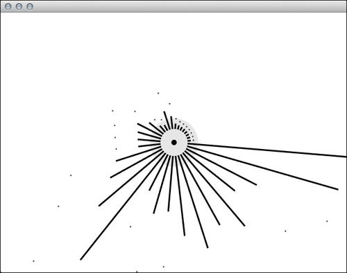
We can divide visualization into bands, and the grey circle with alpha in the center. Bands are straight representations of data calculated by the audio::calculateFft function, and animated with some smoothing by going back towards the center. The grey circle shown in the following screenshot represents the average level of all the bands.
FFT is an algorithm to compute DFT (Discrete Fourier Transform), which decomposes the signal into list of different frequencies.
..................Content has been hidden....................
You can't read the all page of ebook, please click here login for view all page.