
Chapter 5. Relationships between geometries
As the old saying goes, “No man is an island”; the same holds true for geometries. In the previous chapter we concentrated on describing geometries in isolation. We described common properties for geometries and various functions to measure, morph, or transform single geometries. From this chapter forward, we’ll no longer entertain ourselves with one geometry at a time. The richness and the power of spatial queries really come to light when we start working with more than a single geometry. If we liken geometries to tables, an SQL statement that queries from a single table can only go so far. It is only when more than one table gets involved, and we have join operations at our disposal, that things become interesting. Mastery of join operations is what separates the casual database user from the serious database analyst.
Spatial databases have a similar jumping-off point; the casual consumer of a spatial database may use PostGIS to store geometry data or to filter geometries befitting certain conditions. The serious spatial database analyst will be able to write queries that join and morph multiple geometries to solve seemingly intractable problems with brisk elegance.
Although spatial databases are thought of as a tool for geographic information systems, the problems they can tackle aren’t limited to geographic systems. In this chapter we’ll explore the fundamental underpinnings of spatial databases. Spatial databases are all about space—how objects occupy space and interact with other objects in space. Any problem you can state using the physical or abstract concept of vector space is a potential use case for a spatial database. For these exercises we’ll be using the unknown spatial reference system. Later on we’ll delve into spatial reference systems when loading geographic data and cover the special considerations involved with dealing with geographic data.
As the old saying goes, “No pain, no gain.” Working with more than one geometry introduces a new level of conceptual challenges. In non-spatial databases, disparate data interacts through various mathematical or string operations. When one number meets another number, you can add, subtract, multiply, divide, or do some combination thereof. When one string meets another, you can concatenate, or “substring,” one against the other. In spatial databases, when one geometry meets another, things heat up quite a bit. PostGIS has many ways in which the relationship can be consummated. This chapter explores the most commonly used of these relationships. We’ll describe each relationship separately as much as possible in this chapter so that you can gain a solid understanding of what each means. Keep in mind that the full analytical power of spatial SQL usually entails multiple relationship functions, operators, and processing functions being applied in unison.
To avoid muddling meaning while speaking about functions, we suggest that instead of saying ST_SomeRelationship(A,B) say A SomeRelationship B. For example,
ST_Contains(geom1,geom2)
would be read as
geom1 contains geom2
5.1. Introducing spatial relationship functions
Spatial relationship functions in PostGIS accept two input geometries and return either true or false or another geometry. As the name implies, relationship functions describe how the two input geometries relate to each other spatially. For example, if you want to see if one geometry encloses another, you could use ST_Contains. If you want to see if two geometries rub up against each other, you could use ST_Touches.
Not all relationship functions are commutative. Reversing the order of geometries in non-commutative relationships is a fairly common mistake. For instance, if you want to know if A contains B, reversing the input arguments will give you exactly the opposite answer. The exception is invalid geometries, which often return false regardless of the spatial relationship.
When using spatial relationship functions, the two geometries being compared must both be in either the same spatial reference system or in the unknown spatial reference system. If they aren’t, the function may return an error. Keep in mind that all spatial relationship functions for the geometry data type presuppose a planar projection (Cartesian coordinates), so when using lon lat data (spherical coordinates), use the geography type instead, especially when comparing large areas. The geography data type will model the spatial relationships using a true geodetic model, but it’s not as rich in the number of spatial relationship functions you can use with it. For small areas, the Cartesian spatial relationship assumptions will generally work fine, but as the degree differences increase or you approach the poles, treating lon lat as flat is no longer correct, and you may end up with incorrect results.
Although you can create geometries with X, Y, Z, M, and curved geometries in PostGIS, as far as relationships go (those that return true/false), PostGIS currently ignores the third and fourth dimensions, whereas the GEOS relationship functions reject curved geometries.
However, the geometry relationship output functions like ST_Intersection, ST_Difference, and ST_SymDifference don’t completely ignore the Z coordinate, but they apply the Z coordinate after doing a 2D relationship process. The results are sometimes less than desirable.
As a workaround for the lack of support for curves, you can approximate a curve with a non-curve by converting to non-curve and then applying the relationship ST_Intersects(ST_CurveToLine(a.the_geom,100), ST_CurveToLine(b.the_geom, 100)), where 100 is the number of segments to approximate a quarter circle; the default is 32. The 3D issue is harder to compensate for, but PostGIS 2.0 offers new relationship functions specifically designed for 3D.
We start with intersections, because this is by far the most commonly used relationship between two geometries.
5.2. Intersections
The idea of intersection encompasses a wide range of ways in which geometries can interact. We’ll delve into the nuances in time, but let’s start with the basic definition of intersection: Two geometries intersect when they share space.
PostGIS has two functions that work with intersections. The first is ST_Intersects. It takes two geometries and returns true if any part of those geometries is shared between the two. The other function is ST_Intersection. This function returns a geometry that represents the shared part of the two input geometries. If the geometries don’t intersect, then the intersection is an empty geometry. Both functions are defined in the OGC/SQL-MM specs and so can be found in most databases that follow the ISO SQL-MM model.
An empty geometry is a geometry with no points, but it isn’t NULL. You can create an empty geometry by this command: ST_GeomFromText('GEOMETRYCOLLECTION EMPTY'),. Although you can have an empty polygon, PostGIS silently converts it to an empty geometry collection. In version PostGIS 2.0, an empty polygon will return an empty polygon instead of an empty geometry collection.
We’ll demonstrate the two functions in action with some examples.
5.2.1. Segmenting linestrings with polygons
In listing 5.1, we start with a polygon and a linestring and see if they intersect and what the resultant geometry looks like. This example is quite common in real-world scenarios. The linestring can represent the planned route for a new roadway. The polygon can represent private property. Our query quickly tells us whether the new road will cut through the private property. If so, we can determine which part of the road falls within the boundaries to determine the cost associated with an eminent domain takeover. Although we show only a simple example, you can imagine how useful this can be if you have all the private properties in a city and want to determine which properties the road will cut through. The route planner can virtually trace any path through the city and obtain an immediate calculation for the eminent domain purchase.
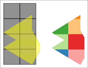
Figure 5.1 shows a planned roadway (linestring), our land mass (polygon), and the resulting intersection geometry—the portion we need to take over by eminent domain.
Figure 5.1. The first image is the POLYGON (our property) overlaid with the LINESTRING (our planned road), and the second is the intersection of the two. This results in a MULTILINESTRING that represents the portion of the property we need to take over.

The code to generate these images is as follows:
SELECT ST_Intersects(g1.geom1,g1.geom2) As they_intersect,
  GeometryType(
  ST_Intersection(g1.geom1, g1.geom2)) As intersect_geom_type
FROM (SELECT ST_GeomFromText('POLYGON((2 4.5,3 2.6,3 1.8,2 0,
  -1.5 2.2,0.056 3.222,-1.5 4.2,2 6.5,2 4.5))') As geom1,
ST_GeomFromText('LINESTRING(-0.62 5.84,-0.8 0.59)') As geom2) AS g1;
In this code we end up with a MULTILINESTRING, as shown in table 5.1, because the line is cut by the polygon.
Table 5.1. Result of query in previous code
|
they_intersect |
intersect_geom_type |
|---|---|
| t | MULTILINESTRING |
Should you be unimpressed by the previous example, the next one ought to change your mind.
5.2.2. Clipping polygons with polygons
One of the most common uses of the ST_Intersection function is to clip polygons. Clipping loosely refers to the process of breaking up a geometry into smaller segments or regions. For instance, if you were in charge of sales for a city and had a dozen sales representatives on your staff, you could clip the polygon of the city into 12 sales regions, one for each representative. Another common use is to make your spatial database queries faster by breaking up your geometries beforehand. If you have data covering more area than you generally need to work with, you can clip the original geometry so as to query against a smaller geometry. For example, if you’re working with data covering the entire island of Hispaniola but only need to report on Haiti, you could clip the island using a linestring and so only query against the data covering the Haitian half of the island. We start with an example where we break up an arbitrarily shaped polygon (the one we used in section 5.2.1) into square regions, as shown in figure 5.2. In order to perform this trick we take a rectangle, break it into eight equal-size cells, and then intersect with our starting polygon, as shown in the following listing.
Figure 5.2. Result of code in listing 5.1. The first image shows a region overlaid against square tiles. The second shows the result of intersection of square tiles with the region.
Listing 5.1. Return our sales region diced up

We ![]() use the PostgreSQL generate_series to generate two series from min/max x and min to max y and skip every two steps so each
square is two units wide and high.
use the PostgreSQL generate_series to generate two series from min/max x and min to max y and skip every two steps so each
square is two units wide and high. ![]() This represents the region we want to cut.
This represents the region we want to cut. ![]() We combine the two and take the intersection, which results in our geometry being diced.
We combine the two and take the intersection, which results in our geometry being diced.
The well-known text representation of each slice is shown in table 5.2.
Table 5.2. The result of the last query in listing 5.1
|
grid_xy |
intersect_geom |
|---|---|
| 0 0 | POLYGON((0.5 0.942857142857143 ......)) |
| 2 0 | POLYGON((2.5 0.9,2 0,0.5 0.942857142857143,0.5 2,2.5 2,2.5 0.9)) |
| 0 2 | POLYGON((-1.18181818181818 2,-1.5 2.2,..)) |
| 2 2 | POLYGON((2.26315789473684 4,2.5 3.55,...)) |
| 0 4 | POLYGON((-1.18179959100204 4,-1.5 4.2,0.5 5....)) |
| 2 4 | POLYGON((2 4.5,2.26315789473684 4,0.5 4,0.5 5.51428571428571...)) |
| 2 6 | POLYGON((1.23913043478261 6,2 6.5,2 6,1.23913043478261 6)) |
This example shows how intersections can be useful for partitioning a single geometry into separate records. Notice that the cutting squares don’t need to completely cover the polygon. In this case we left out the last sliver by making our grid not completely cover the extent of the region.
Another important thing to keep in mind is that the geometry type returned by ST_Intersection may look rather different than the input geometries, but it’s guaranteed to be of equal or lower dimension than the lowest dimension geometry. For example, if you have two polygons that share an edge, then the intersection of the two will be the linestring representing the shared edge. Similarly, if you intersect a road with a parcel of land, then the intersection would be possibly a linestring that represents the portion of the road that runs through the parcel of land.
To summarize, if A and B are the input geometries to ST_Intersection, then the following are true:
- ST_Intersection returns the portion shared by A and B.
- ST_Intersection and ST_Intersects are both commutative—meaning that ST_Intersection(A,B) = ST_Intersection(B,A) and ST_Intersects(A,B) = ST_ Intersects(B,A).
- A and B need not be of the same geometry type.
- The geometry returned by ST_Intersection is of equal or lower dimension of the lowest dimensioned of both input geometries.
- If A and B don’t intersect, then the intersection is an empty geometry.
Now that we’ve covered the basic concept of intersects and intersection, we’ll delve into the finer details of intersecting relationships.
5.3. Specific intersection relationships
Recall that the definition of intersection involves two geometries sharing space. Sometimes, you may want to have more detail about how the space is shared and have to say something about the space not being shared. For these situations, you have at your disposal many PostGIS functions that focus on the properties of the intersection. Again, these functions rely on the fact that the spatial reference system (SRS) of both geometries is the same, though their geometric dimensions need not be the same. The geometries should also be valid; otherwise, the results can’t be trusted.
5.3.1. Interior, exterior, and boundary of a geometry
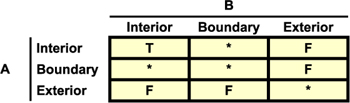
Most of the intersection relationship functions rely on the concepts of interior, exterior, and boundary of a geometry and whether these intersect with the interior, exterior, and boundary of the second geometry. In the case of intersection of these three parts, the geometric dimension of the resulting geometry is also important. Will the intersection result in a geometry of zero, one, or two dimensions?
We’ll cover these concepts in more detail in a later section of this chapter. For brevity, this is what the terms mean:
- Interior— That portion of a geometry that’s inside the geometry and not on the boundary.
- Exterior— The coordinate space outside a geometry but not including the boundary.
- Boundary— The coordinate space neither interior nor exterior to the geometry. It’s the space that separates the interior from the exterior (the rest of the coordinate space). Recall that we covered in the prior section ST_Boundary, which tells the boundary geometry of a geometry.
The boundary of a geometry is another geometry. In the case of finite points, the boundary is an empty geometry. You can get the boundary of a geometry with the ST_Boundary function, and this resultant geometry also has an interior, exterior, and boundary. The model of an interior and exterior is a bit harder to fathom without introducing the concept of limit theorems. You can’t adequately represent it with a geometry construct except in the case of interior for points and multipoints. The interior of points is simply the points, and the exterior is the rest of the coordinate space that’s not the points. In the case of lines and polygons, the interior and exterior are limits approaching the boundary of the geometry and therefore not representable by themselves. In short, the model of a geometry is a mathematical trick. In the case of linestrings and polygons, we can’t quantify what an interior is or an exterior is, but we can say there exists an object called a “geometry” composed of an infinite number of points that has an interior, an exterior, and a boundary, where the interior and exterior approach the boundary.
The result of an intersection of these nine pairs can be non-dimensional (no intersection), zero dimensional (finite points), one dimensional (lineal), two dimensional (areal polygons), or a combination thereof in which the dimension is the dimension of the highest dimension element in the collection.
These intersect classes of functions should be used only with valid geometries. The reason is that when there are self-intersections at the boundaries, the concepts of interior, exterior, and boundary are not well defined. This is a common mistake.
The official PostGIS manual has diagrams of these relationships. We’ll try to focus on the corner cases where people have a hard time comprehending the relationships.
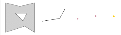
We’ll use the house example shown in figure 5.3 for explanation of specific intersection relationships because it’s a simple corner case that exercises the subtleties of all these relationships.
Figure 5.3. A shaded polygon with a hole (a house with a courtyard), a linestring (a walkway), a multipoint represented as two dots (two greeters: front door and courtyard greeter), and a point as a triangle (a door) generated from the code in listing 5.2
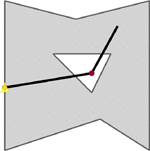
When these geometries are viewed together on the same grid, the overlay looks like figure 5.4.
Figure 5.4. The polygon with a hole (a house with a courtyard), the linestring (a walkway), the multipoint (two greeters), and the point as a triangle (a door) seen together. All are generated from the code in listing 5.2.
In this example, we have four geometries that we can envision as any set of objects:
- A polygon with a triangular hole—This is our house with a courtyard. The courtyard we represent as a hole because we don’t consider it part of the house. The courtyard is thus geometrically a part of the house’s exterior.
- A linestring—This can be a red carpet for visitors to walk into the house.
- A point represented by a triangle icon—This is the front door to our house.
- A multipoint represented by two dots—This can be two greeters who are stationed at the front door to greet incoming visitors and at the courtyard to seat guests.
At a particular moment in time, we see all these objects at these particular positions.
We create this particular dataset with the following piece of code.
Listing 5.2. Create sample geometries to exercise intersect relationships
CREATE TABLE example_set(ex_name varchar(150) PRIMARY KEY,
    the_geom geometry);
INSERT INTO example_set(ex_name, the_geom)
VALUES
('A polygon with hole',
    ST_GeomFromText('POLYGON ((110 180, 110 335,
     184 316, 260 335, 260 180, 209 212.51, 110 180),
(160 280, 200 240, 220 280, 160 280))') ),
('A point',ST_GeomFromText('POINT(110 245)')) ,
('A linestring',
    ST_GeomFromText('LINESTRING(110 245,200 260, 227 309)')) ,
('A multipoint',
     ST_GeomFromText('MULTIPOINT(110 245,200 260)')) ;
Next we’ll look at Contains and Within.
5.3.2. Contains and Within
Contains and Within are companion relationships. If geometry A is within geometry B, then geometry B contains geometry A. The Within and Contains relationships are supported by the PostGIS ST_Within and ST_Contains functions. Both of these functions are OGC/SQL-MM–defined functions, so they can be found in other spatial databases. They have more or less the same meaning in all spatial databases.
One of the confusing but necessary conditions for geometry A to contain geometry B is that the intersection of the boundary of A with B can’t be B. In other words, B can’t sit entirely on the boundary of A. A geometry doesn’t contain its boundary, but a geometry always contains itself.
With the following query we can answer such fascinating questions as, are both greeters inside the house and not in the courtyard? Are they both on the walkway? Is one still at the front door?
SELECT A.ex_name As a_name, B.ex_name As b_name,
     ST_Contains(A.the_geom, B.the_geom) As a_co_b,
     ST_Intersects(A.the_geom, B.the_geom) As a_in_b
FROM example_set As A CROSS JOIN example_set As B;
The result of this code is shown in table 5.3.
Table 5.3. Result of the query: All intersect but not all contain.
|
a_name |
b_name |
a_co_b |
a_in_b |
|---|---|---|---|
| A polygon with hole | A polygon with hole | t | t |
| A polygon with hole | A point | f | t |
| A polygon with hole | A linestring | f | t |
| A polygon with hole | A multipoint | f | t |
| A point | A polygon with hole | f | t |
| A point | A point | t | t |
| A point | A linestring | f | t |
| A point | A multipoint | f | t |
| A linestring | A polygon with hole | f | t |
| A linestring | A point | f | t |
| A linestring | A linestring | t | t |
| A linestring | A multipoint | t | t |
| A multipoint | A polygon with hole | f | t |
| A multipoint | A point | t | t |
| A multipoint | A linestring | f | t |
| A multipoint | A multipoint | t | t |
The example brings to light the following items:
- All the above objects intersect each other. This tells us at least one greeter is at the front door, at least one greeter is on the walkway, and at least one greeter is wholly within the confines or on the boundary of the house (but they can’t both be in the courtyard because they as a whole would not intersect the house if they were both in the courtyard).
- Because the polygon (house) does not contain the multipoint (the greeters), but the greeters intersect the house, we know that one person must be in the courtyard or outside the outer boundary of the house. We know that the pathway is not completely in the house but intersects it—it must have some piece that’s in the courtyard or that sticks out of the house.
- If geometry B sits wholly on the boundary of geometry A, geometry A doesn’t contain geometry B. Because the point (door) intersects the house but the house doesn’t contain the door, we know the door must be on the boundary of the house. The door intersects the linestring (walkway) but the walkway doesn’t contain the door; therefore the door must be on the boundary of the walkway (at the start point or the end point of the walkway). The walkway contains both people; therefore at most one person can be at the start or end of the walkway but not both.
- All geometries contain themselves (a multipoint (the greeters) contains itself, a linestring (walkway) contains itself, and so on).
If we were to use ST_Within, it would just be the inverse of ST_Contains—just flip the A and B geometry columns.
5.3.3. Covers and CoveredBy
As you’ve observed from the Contains example, the concept of OGC/SQL-MM containment is non-intuitive at the boundaries. Most people make the mistake that a geometry should contain its boundary points, and that’s an often-desired feature. This is why PostGIS introduced the concept of Covers and CoveredBy to satisfy this need that interestingly enough also exist in Oracle Spatial via the SDO_RELATE mask=COVEREDBY construct. These functions are called ST_Covers and ST_CoveredBy in PostGIS, and they are not OGC/SQL-MM defined functions. Here are a couple of other caveats:
- These functions rely on functionality introduced in GEOS 3.0, so if you happen to be running, say, PostGIS 1.3 compiled with GEOS < 3, you won’t have these functions available.
- ST_Covers is exactly like ST_Contains except it will also return true in the case where a geometry lies completely in the boundary of the other. ST_CoveredBy is to ST_Covers as ST_Contains is to ST_Within.
The following listing and table 5.4 demonstrate situations where ST_Covers covers a geometry but does not contain it.
Table 5.4. Result of query in listing 5.3: List all where the answer of Covers is different from that of Contains.
|
a_name |
b_name |
a_co_b |
a_in_b |
|---|---|---|---|
| A polygon with hole | A point | t | t |
| A linestring | A point | t | t |
Listing 5.3. How is ST_Covers different from ST_Contains?
SELECT A.ex_name As a_name, B.ex_name As b_name,
    ST_Covers(A.the_geom, B.the_geom) As a_co_b,
    ST_Intersects(A.the_geom, B.the_geom) As a_in_b
FROM example_set As A CROSS JOIN example_set As B
WHERE NOT (ST_Covers(A.the_geom, B.the_geom) =
  ST_Contains(A.the_geom, B.the_geom));
In this code we’re going to list only those geometries where the ST_Covers answer is different from the ST_Contains answer. Table 5.4 shows the result of this query.
Because we limited our result to the case where the answer produced by ST_Covers is different from that of ST_Contains, A is considered to cover B even in the case where a geometry sits wholly on the boundary of A. Both the walkway and the house cover the door, but they don’t contain the door.
5.3.4. ContainsProperly
ContainsProperly is a concept that’s more stringent than the Contains or Covers relationships. Its main benefit is that it’s in general faster to compute than the others, and if you want to exclude geometries that sit partly or wholly on the boundary of another, it’s the one you want. You may want to do this, for example, if you want to make sure your ships are all without a doubt legally within your political boundary.
ContainsProperly will give you the same result as Contains except in the case where any part of geometry B sits on the boundary of A. In listing 5.4 we repeat the same exercise, except that we list only the ContainsProperly options where ST_ContainsProperly gives a different answer from ST_Contains. Here are a couple of caveats to consider:
- It’s not an OGC/SQL-MM–defined function; it’s a PostGIS-specific function.
- It was introduced in PostGIS 1.4.
- It requires GEOS 3.1 or above, so if you’re running PostGIS 1.4 with, say, GEOS 3.0.3, this function won’t be available to you.
Listing 5.4. How is ST_ContainsProperly different from ST_Contains?
SELECT A.ex_name As a_name, B.ex_name As b_name,
    ST_ContainsProperly(A.the_geom, B.the_geom) As a_co_b,
    ST_Intersects(A.the_geom, B.the_geom) As a_in_b
FROM example_set As A CROSS JOIN example_set As B
WHERE NOT (ST_ContainsProperly(A.the_geom, B.the_geom) =
   ST_Contains(A.the_geom, B.the_geom));
Table 5.5 shows the result of this query. Observe that ST_ContainsProperly gives an identical answer to ST_Contains except in the case of an areal geometry, a line geometry compared to itself, or a geometry sitting partly on the boundary of another. A geometry never properly contains itself except in the case of points and multipoints. The reason points and multipoints properly contain themselves is that they consist of a finite number of points and therefore have no boundary to speak of. A point can never be sitting partly on its nonexistent boundary.
Table 5.5. Result of query in listing 5.4: geometries where Contains and ContainsProperly are different
|
a_name |
b_name |
a_co_b |
a_in_b |
|---|---|---|---|
| A polygon with hole | A polygon with hole | f | t |
| A linestring | A linestring | f | t |
| A linestring | A multipoint | f | t |
You can see from this that the only cases where the ST_ContainsProperly answer is different from that of ST_Contains are the cases of a polygon against itself, a linestring against itself, or a point or multipoint that partly sits on the boundary of another. This tells us one person must be on the start or end of the walkway because the walkway doesn’t properly contain both people, but it does contain both people.
5.3.5. Overlapping geometries
Two geometries overlap when they’re the same geometric dimension (points, areal, linestring), they intersect, and one is not contained in another. The function that supports overlaps in PostGIS is called ST_Overlaps. This function is an OGC/SQL-MM–compliant function. If we used the same example as we used previously, comparing if each one overlaps the other, we’d find that none overlap. The reasons for that are as follows:
- The linestring (walkway) as we’ve modeled it is not of the same dimension as the polygon (house), so it can’t overlap, and the same holds true with point/ polygon (door/house) and point/linestring (door/walkway).
- The multipoint (greeters) can’t overlap with the point (door), because the door is in the same position as a greeter. It is contained and covered by the greeters.
- The line/line, multipoint/multipoint, point/point, and polygon/polygon don’t overlap because each contains itself.
5.3.6. Touching geometries
Two geometries are considered to touch if they have at least one point in common but those points don’t lie in the interior of both geometries. The function that supports this relationship is ST_Touches, and it’s an OGC/SQL-MM–defined function. Revisiting our example of the polygon with a hole (house with a courtyard), linestring (walkway), point (door), and multipoint (front and courtyard greeters), we ask which pairs of these touch. Can you guess?
SELECT A.ex_name As a_name, B.ex_name As b_name,
    ST_Touches(A.the_geom, B.the_geom) As a_tou_b,
    ST_Contains(A.the_geom, B.the_geom) As a_co_b
FROM example_set As A CROSS JOIN example_set As B
WHERE ST_Touches(A.the_geom, B.the_geom) ;
The result of this question is listed in table 5.6.
Table 5.6. Result of latest query: geometries that touch each other
|
a_name |
b_name |
a_tou_b |
a_in_b |
|---|---|---|---|
| A polygon with hole | A point | t | f |
| A polygon with hole | A multipoint | t | f |
| A point | A polygon with hole | t | f |
| A point | A linestring | t | f |
| A linestring | A point | t | f |
| A multipoint | A polygon with hole | t | f |
There are a couple of important points to glean from these results:
- The touch relationship is symmetric (or commutative); if a touches b, then b touches a.
- The house touches the door and the walkway touches the door, because the door lies on the boundary of the house and walkway (not the interior of the house or walkway), even though the shared point is in the interior of the door.
- The multipoint/point pair (people/door) is missing because one contains the other and also the shared point is interior to both geometries. A point can never touch a point or a multipoint because the shared points would always be interior to both.
- The multipoint (people) and the polygon (house) touch because one person of the multipoint is on the boundary of the house and the other is in the hole (courtyard). Note that because we modeled the courtyard as a hole, the courtyard is part of the exterior of the house and not the interior. So even though one greeter is basking in the courtyard and the other is at the door, as a pair they are touching the house.
5.3.7. Crossing geometries
Two geometries are said to cross each other if they have some interior points in common but not all. The function that supports crosses is ST_Crosses, and it’s an OGC/ SQL-MM–defined function.
Revisiting our example of the polygon with a hole (the house with a courtyard), linestring (walkway), point (door), and multipoint (front door and courtyard greeters), we ask which pairs of these cross. Can you guess?
SELECT A.ex_name As a_name, B.ex_name As b_name,
    ST_Crosses(A.the_geom, B.the_geom) As a_cr_b,
    ST_Contains(A.the_geom, B.the_geom) As a_co_b
FROM example_set As A CROSS JOIN example_set As B
WHERE ST_Crosses(A.the_geom, B.the_geom) ;
The result of this question is listed in table 5.7.
Table 5.7. Result of this query: geometries that cross each other
|
a_name |
b_name |
a_cr_b |
a_co_b |
|---|---|---|---|
| A polygon with hole | A linestring | t | f |
| A linestring | A polygon with hole | t | f |
We can glean a few things from this example:
- We have only one pair of geometries that cross each other: the linestring (walkway) and the house. The reason these cross is that they don’t touch or contain each other but they do intersect. The shared region contains points interior to both, but one is not completely contained by the other. Note that this touching is made possible by the hole (the courtyard). The walkway has some points that fall within the courtyard, so its interior is not completely contained by the house’s interior.
- None of our touch winners are crossing winners. If you touch, you can’t cross.
- It’s okay for boundary points to be shared.
5.3.8. Disjoint geometries
The Disjoint relationship is the antithesis of Intersects. It means the two geometries have no interiors or boundaries shared. In the case of invalid geometries, it’s possible for the ST_Intersects and ST_Disjoint functions to both return false. If you see such a thing, you know your geometry is invalid.
The disjoint relationship is supported by the function ST_Disjoint, and it too is an OGC/SQL-MM–defined function.
Now that we’ve covered all the many facets of intersects and intersection, in the next section we’ll take a look at output functions that are very closely related to Intersection. These are the Difference family of functions.
5.4. The remainder: ST_Difference and ST_SymDifference
Two output relationship functions are very closely related to Intersection and Intersects. These are Difference and Symmetric Difference. These are much less commonly used than ST_Intersection and return the remainder of an intersection. ST_Difference is a non-commutative function whereas Symmetric Difference is, as the name implies, commutative.
Symmetric Difference is the dark twin of the intersection. It will return the simplest geometric representation of what’s
left out when two geometries form an intersection. The ST_Difference function when given a geometry A and B ![]() ST_Difference(A,B) returns that portion of A that’s not shared with B.
ST_Difference(A,B) returns that portion of A that’s not shared with B.
Here’s one way to think about it:
ST_SymDifference(A,B) =  Union(A,B) - Intersection(A,B)
ST_Difference(A,B) = A - Intersection(A,B)
In the following listing we repeat a similar exercise to the one we did with Intersection except we’re computing a Difference instead of an Intersection.
Listing 5.5. What’s left of the polygon and line after clipping

![]() This results in a polygon, which is pretty much the same polygon we started out with. This may be surprising to some; you’d
expect a linestring would split it.
This results in a polygon, which is pretty much the same polygon we started out with. This may be surprising to some; you’d
expect a linestring would split it. ![]() This results in a multilinestring composed of three linestrings where the polygon cuts through.
This results in a multilinestring composed of three linestrings where the polygon cuts through. ![]() Finally, this results in a geometry collection as expected, composed of a multilinestring and a polygon.
Finally, this results in a geometry collection as expected, composed of a multilinestring and a polygon.
Figure 5.5 is a diagram of the results.
Figure 5.5. Queries from listing 5.5 output. Observe that the difference of the polygon and the line is pretty much the polygon we started out with.

As you can see, the linestring doesn’t bisect the polygon, though this is a common desire in many cases. Why? If you think of a geometry as an infinite set of points, the difference caused by the linestring would be two polygons with partially shared boundaries. The simplest geometry to describe them is the union of these polygons, which is more or less the original polygon, not a geometry collection of two polygons or a multipolygon. It can’t be a multipolygon because a valid multipolygon can’t have polygons that intersect at more than one point.
The result you get of the difference of the polygon from the line is not quite the polygon you started out with. It looks like it, but it has one or two point differences at the boundaries where the line cuts through. This is more an artifact of the differencing operation and not because of any theoretical reason.
One not so elegant hack to achieve bisection is to turn the linestring into a thin knife by buffering it ever so slightly, such that the boundaries of the resulting polygons won’t intersect, and then gluing back the leftover slivers onto one of the resulting polygons. This often is good enough in many cases. The following listing is such a demonstration minus the glue. Table 5.8 and figure 5.6 show the result.
Figure 5.6. Result of the knife trick in listing 5.6

Table 5.8. Query result of listing 5.6: The polygon is cut into three parts.
|
gid |
wktpoly |
|---|---|
| 1 | POLYGON((2 4.5,3 2.6,3 1.8,2 0,-0.760732 1.7353172,...-0.6572407 4.7538133,2 6.5,2 4.5)) |
| 2 | POLYGON((-0.760732 1.7353173,-1.5 2.2,-0.7274017 2.7074521,-0.760732 1.7353173)) |
| 3 | POLYGON((-0.6936062 3.6931535,-1.5 4.2,-0.6572407 4.7538133,-0.6936062 3.6931535)) |
Listing 5.6. Bisecting a polygon using the knife trick
SELECT foo.path[1] As gid,
 ST_AsText(
  ST_SnapToGrid(foo.geom, 0.0000001)) As wktpoly
FROM (SELECT g1.geom2 As the_knife_cut,
  (ST_Dump(ST_Difference(g1.geom1, g1.geom2))).*
FROM
  (SELECT
ST_GeomFromText('POLYGON((2 4.5,3 2.6,3 1.8,2 0,
 -1.5 2.2,0.056 3.222,-1.5 4.2,2 6.5,2 4.5))') As geom1,
ST_Buffer(
 ST_GeomFromText('LINESTRING(-0.62 5.84,-0.8 0.59)'),0.00000001) As geom2) AS g1
WHERE ST_Intersects(g1.geom1,g1.geom2)) As foo;
As you can see in this example, we buffer the line to make it a very thin polygon we can cut with. This cuts the polygon into three, resulting in a multipolygon, which we then break apart into three polygons using the ST_Dump function you learned about in the previous chapter. In later sections we’ll delve into more precise but advanced options of cutting geometries.
PostGIS 2.0 added the ST_Split function, which allows for splitting a line by a point, line by line, or polygon by line with a single statement. All these can be done much simpler and more exact using ST_Split.
In the coming sections we’ll explore the ST_DWithin relationship function that you’ve seen in earlier examples. It’s very closely related in functionality to ST_Intersects.
5.5. Nearest neighbor
We briefly covered the ST_DWithin function in chapter 1. In this section, we’ll cover some more examples of its usage.
ST_DWithin, as mentioned earlier, is used most commonly to find geometries that are close to another or determine if a geometry is within X units of another. This process is often called a nearest neighbor search. In versions of PostGIS prior to 1.3.5, this was shorthand for ST_Expand(A,X) && B AND ST_Expand(B,X) && A AND ST_Distance(A,B) < X.
These expand calls may seem redundant: If one is true then both are true, and if one is false then both are false. The reason both are needed is that depending on how you expand you may end up using an index or not, and SQL planners don’t process statements in order. They first try to process statements in order of cost when computing costs are not more costly than sequential. At runtime one of those checks is generally far more costly than another because one is generally a constant geometry (that’s the one you’d want to expand) and the other is a table with a spatial index on the geometry, which if you expand it will no longer use the spatial index. The planner will choose the least costly way to process the first, so only in the case of positives will the second call be made. Also keep in mind that ST_Expand expands the bounding box, not the geometry, and so returns a box. You can think of ST_Expand as the lazy sibling of ST_Buffer.
From PostGIS 1.3.5 on, additional short-circuit logic is built in.
The ST_DWithin is not an MM/SQL function, but it’s pseudo standards compliant in that the many Web Feature Services (WFS) such as GeoServer, MapServer, MapInfo WFS, and Deegree have a DWithin filter operator that does the same thing. Oracle also has a function called SDO_GEOM.WITHIN_DISTANCE that operates the same way, except the Oracle version accepts a unit of measure as argument, whereas the PostGIS one always assumes the units are the units defined for the spatial reference system of the geometries.
5.5.1. Intersects with tolerance
Another side use of this function is as a substitute for the ST_Intersects function. This usage we term as doing an intersects with tolerance.
Here are a few reasons why you may choose to use this function instead of the more obvious ST_Intersects:
- Because of rounding errors, your geometries are really close but they don’t intersect. If, for example, you take the point on surface of a line, often that point will no longer intersect the line it came from. In these cases you can treat ST_DWithin as a more forgiving Intersects, or as we like to call it ST_Intersects with tolerance, by providing a distance that’s very small.
- ST_DWithin doesn’t choke on invalid geometries as ST_Intersects often does. With ST_Intersects you’ll often get a topology intersects exception error if your geometry has self-intersecting regions. ST_DWithin doesn’t care because it doesn’t rely on an intersection matrix.
- Although ST_DWithin doesn’t work with curved geometries as of PostGIS 1.5, you can expect it to do so in later versions, possibly even in a minor release. This is because ST_DWithin is a native function of PostGIS and ST_Intersects is a GEOS function.
When used in this manner, the distance parameter must be set to very small to represent the maximum distance error to consider two geometries as intersecting. For example, you may consider the linestring and a point to be intersecting if they’re within 0.01 units of each other:
SELECT
    ST_DWithin(
        ST_GeomFromText('LINESTRING(1 2, 3 4)'),
            ST_Point(3.00001,4.000001),
        0.0001
 ) ;
Next we’ll look at finding the N closest objects.
5.5.2. Finding N closest objects
There are many ways of doing a nearest neighbor search. The classic example is finding, for example, the nearest five roads to a particular location that are within 10 kilometers of the location:
SELECT r.name, ST_Distance(r.geom, loc.geom)/1000 As dist_km
    FROM ch01.roads As r INNER JOIN
    (SELECT ST_Transform(
       ST_SetSRID(ST_Point(-118.42494, 37.31942), 4326),
         2163) As geom) As loc
  ON ST_DWithin(r.geom, loc.geom, 10000)
ORDER BY ST_Distance(r.geom, loc.geom)
    LIMIT 5;
In this example we’re concerned only with finding roads near a single point. The location needn’t be a point; it can just as well be a lake, a river, or a building that’s represented as a linestring or a polygon or even a geometry collection. Here we’re assuming our table geometries are stored in US National Atlas Equal Area meter projection (2163) and our point of interest is in lon lat (4326), so we transform to (2163) to do a meter-based search. The ST_DWithin check as described in earlier chapters returns true if any point on geometry A is within X distance of any point on geometry B. The X is always in the units of the spatial reference system of those geometries, and the SRID of the two geometries must be the same.
As you’ll note, with ST_DWithin you need to provide a limit distance. If you wanted to find the five closest roads, doing a simple order by ST_Distance(....) limit 5 without the ST_DWithin, it would be very slow because the query would resort to what’s called a table scan—calculating the distance of loc to every geometry in the table and returning the five closest. ST_DWithin reduces the set of false positives significantly. Thus it requires that you know something about your data—that you know all the top five geometries are within 10 kilometers. The less you know about your data, the larger you should make your X, and in return the slower your query will become because it will grab more false positives to inspect. Some of this will change in PostgreSQL 9.1/ 9.2 and PostGIS 2.0+ because k nearest neighbors (kNN) scanning will be added to GIST indexes in PostgreSQL 9.1 or PostgreSQL 9.2 that may make this exercise much easier and efficient.
Another common use case is to find the closest from some other geometry. For this kind of query the DISTINCT ON custom SQL addition of PostgreSQL in conjunction with ST_DWithin comes in very handy. Listing 5.7 is a classic example of its use. DISTINCT ON is guaranteed to return at most one record for any DISTINCT set defined in the ON part. In this example we do the same as previously, except we do it for all locations of interest and return the closest road to each location of interest.
Listing 5.7. Find the closest road to each location; search 10 kilometers out
SELECT DISTINCT ON(loc.loc_name, loc.loc_type) loc.loc_name,
    loc.loc_type, r.road_name,
        ST_Distance(r.the_geom, loc.geom)/1000 As dist_km
FROM ch05.loc LEFT JOIN
        ch05.road As r
ON ST_DWithin(r.the_geom, loc.geom, 10000)
ORDER BY loc.loc_name, loc.loc_type,
  ST_Distance(r.the_geom, loc.geom) ;
There are three important things about using DISTINCT ON:
- The ON(...) can have many fields that uniquely identify the record you want to be distincted, but these must appear in the ORDER BY and be the first fields to appear in the ORDER BY.
- In the ORDER BY you can add additional columns in addition to the DISTINCT ON ones, to control which record gets picked as the unique one.
- Observe that we changed our query to be a LEFT JOIN; this is so that all loc_name, loc_city combos are returned even if there’s no road within 10 kilometers. If you didn’t care or were sure all would have roads that close, you could get better performance by making this an INNER JOIN.
5.5.3. Using SQL Window functions to number results
Sometimes you want n nearest neighbors for each of your location records; sadly neither DISTINCT ON nor the LIMIT clause will let you do this in one query. Luckily Post-greSQL 8.4 has what are called Window functions. Window functions are an ANSI SQL 2003 standard piece you’ll find in all the high-end enterprise-class commercial databases (Oracle, IBM DB2, and SQL Server 2005/2008). The windowing support in PostgreSQL is more feature rich than in SQL Server 2005/2008, but it’s not quite as feature rich as what you’ll find in Oracle or IBM DB2. Read the SQL Primer appendix for more details of what ANSI windowing functionality is supported and what is not.
The following example requires PostgreSQL 8.4. It will return the top five closest roads for each location of interest that are within 20 kilometers.
Listing 5.8. Find the closest two roads to each station; search 1 kilometer out.

This query is run against the fictitious poorly designed town we demonstrated at Post-greSQL Conference 2009 (PGCON2009). The code to build the town is available for download from http://www.postgis.us/presentations. The dataset already built is included in the chapter 5 code data download.
Table 5.9 shows a sampling of the results. There are three important things to take away from this example:
Table 5.9. Results of query in listing 5.8
|
Pid |
land_type |
row_num |
road_name |
dist_km |
|---|---|---|---|---|
| 000001038 | police station | 1 | ||
| 000001202 | police station | 1 | ||
| 000002997 | police station | 1 | Main Rd | 0.25 |
| 000003927 | police station | 1 | Main Rd | 0.07 |
| 000006442 | police station | 1 | ||
| 000010131 | police station | 1 | Main Rd | 0.23 |
| 000010131 | police station | 2 | Curvy St | 0.34 |
| 000013872 | police station | 1 | ||
| 000015423 | police station | 1 | Elephantine Rd | 0.45 |
- The windowing function ROW_NUMBER() will create sequentially numbered rows for each partition defined in the PARTITION BY of the OVER clause and restart numbering at the next partition (here we’re partitioning by the parcel id), and the rows will be numbered by what we specify in the ORDER BY of the OVER clause, in this case Distance to a road.
- We’re using a left join, which guarantees that all records in our WHERE will be included—in this case all police stations—but only roads within one kilometer of each police station will be considered.
- We then order the final result by parcel id and then the proximity of road, which is our row_num (the result of our ROW_NUMBER() windowing call).
Table 5.9 lists partial results from our query. Observe that for police stations farther than one kilometer from a road, we still get back a record—but the street slots are filled in with NULLs. Some police stations have more than one road within one kilometer (for example, 000010131), and for that one we get two records back with the first including the closest road and the second the next closest.
Now that we’ve covered the basics of proximity analysis, we’ll move on to bounding boxes and basic geometry comparators. Although we didn’t stress it in this section, what makes proximity queries fast are the box-based short-circuit comparisons. Bounding boxes and their geometry operators are used by spatial indexes to reduce the set of records that need to be more closely scrutinized by the exact comparison operators. We’ll cover this in the next section.
5.6. Bounding box and geometry comparators
Recall from the previous chapter that every geometry has a bounding box, defined as the smallest rectangular box that completely encloses the geometry. Bounding boxes play a critical role when two geometries interact. Now that we’ve covered the basics of proximity analysis, we’ll move on to bounding boxes and basic geometry comparators.
5.6.1. The bounding box
Let’s demonstrate with a quick example. Suppose we have two multipolygons, one representing the state of Washington and one representing the state of Florida. If the bounding box of Washington is strictly above and to the left of (northwest of) Florida, then we know for sure that the actual geometries share the same relationship as well. Of course, if the bounding boxes check is false, we can’t be sure. Remember now that both states have numerous islands hanging off their coasts. In order to answer the questions unequivocally, we’d have to pretty much visit every point in Washington and compare it to every point in Florida. Only after this exhaustive point-by-point checking could we conclude that all of Washington is northwest of all of Florida. The bounding box methodology shortcuts the point-by-point checking by first drawing rectangular boxes around each state and then asking if the box enclosing Washington is above and to the left of the box enclosing Florida. We can obtain an answer almost instantly. Furthermore, because a rectangular box is completely specified by the coordinate of two opposing corners, we can pre-calculate all the bounding boxes for geometries in our table and store their coordinates in indexes. Once we have the bounding box of every geometry indexed, comparing any two geometries becomes a simple task of comparing two pairs of numbers.
Bounding boxes are so fundamental to the spatial queries that PostGIS always assumes that you’d take advantage of them, freeing you from having to worry about explicitly calculating bounding boxes and creating indexes out of them.[1] Certainly, we can foresee many instances where bounding boxes won’t do us much good in the end. Suppose we want to know if the centroid of Washington State is to the left of the centroid of Oregon; we can’t shortcut ourselves to an answer by simply looking at the bounding box of the two states. The next listing contains examples of geometries with their bounding boxes wrapped around them.
1 The only exception is when you use deprecated functions.
Listing 5.9. ST_Box2D and geometry
SELECT ex_name, ST_Box2D(the_geom) As bbox2d, the_geom
FROM (
VALUES
 ('A line', ST_GeomFromEWKT('LINESTRING (3 5, 3.4 4.5, 4 5)')),
('A multipoint',ST_GeomFromText('MULTIPOINT (4.4 4.75, 5 5)')) ,
('A triangle', ST_GeomFromText('POLYGON ((2 5, 1.5 4.5, 2.5 4.5, 2 5))') )
)
AS foo(ex_name, the_geom);
Figure 5.7 illustrates the output of this query, showing the geometries encased in their bounding boxes.
Figure 5.7. Various geometries and their bounding boxes from geometries in listing

For brevity we stated that the bounding box is the smallest box you can wrap around a geometry. Strictly speaking, it’s not the smallest. PostGIS will often expand a bounding box to ensure that the coordinates can be represented with float4 numbers. For example, if the smallest box is defined by the two corners of (-3.14159265,0) and (0,2.71828182), PostGIS may round this off to (-3.15,0) and (0,2.72). The size limit of the box coordinates may change in future versions.
5.6.2. Bounding box and geometry operators
PostGIS offers a number of geometry bounding box comparators that work exclusively with box2d objects and one comparator that works against the actual geometry. Some but not all of these operators have functional counterparts that apply to the entire geometry. As a convenient shorthand, PostGIS uses various operators to symbolize comparators. For example, A && B returns true if bounding box of geometry A intersects bounding box of geometry B or vice versa where the double ampersand operator (&&) is the intersection comparator. The && operator is the one most commonly used as a precheck for spatial relationships.
Table 5.10 is a quick table of the operators, what they do, and what kind of index they use. Keep in mind that in general you put GIST indexes on geometries. B-tree indexes are possible only if geometry objects are relatively small, such as points or small polygons and lines. If you have no B-tree index, then an operator that works only with B-tree won’t use an index. You can have both a GIST and a B-tree index on the same geometry field; B-tree indexes on geometries are rare and of minimal utility.
Table 5.10. PostGIS operators that can be applied to geometries
|
Operator |
What is checks |
Index |
|---|---|---|
| && | Returns true if A’s bounding box intersects B’s | gist |
| &< | Returns true if A’s bounding box overlaps or is to the left of B’s. | gist |
| &<| | Returns true if A’s bounding box overlaps or is below B’s. | gist |
| &> | Returns true if A’s bounding box overlaps or is to the right of B’s | gist |
| << | Returns true if A’s bounding box is strictly to the left of B’s | gist |
| <<| | Returns true if A’s bounding box is strictly below B’s | gist |
| = | Returns true if A’s bounding box is the same as B’s | B-tree |
| >> | Returns true if A’s bounding box is strictly to the right of B’s | gist |
| @ | Returns true if A’s bounding box is contained by B’s | gist |
| |&> | Returns true if A’s bounding box overlaps or is above B’s | gist |
| |>> | Returns true if A’s bounding box is strictly above B’s | gist |
| ~ - | Returns true if A’s bounding box contains B’s | gist |
| ~= | Obsolete; superseded by ST_OrderingEquals | gist |
Although all the operators are used to compare only bounding boxes (box2d objects), except for the ~= sameness operator, which works against true geometries, all these operators can be called for both plain bounding boxes box objects (box2d) as well as actual geometries. They are generally used with geometries and look at the bounding box wrapper around the geometry.
Now that we’ve covered the basics of bounding boxes, which are used extensively as a precheck for other relationships, we’ll explore the most fundamental relationship: equality and its multifaceted meaning.
5.7. The many faces of equality
In conventional databases, you probably never gave the equality comparator (=) a second thought before using it. This unambiguity doesn’t carry over to spatial databases. When we compare two geometries, equality is a multifaceted notion. We can ask whether geometries occupy the same space. We can ask whether they are represented by the same points. We can ask whether their bounding boxes are the same.
Three basic kinds of equality are specific to geometries in PostGIS:
- Spatial equality (occupying the same space)
- Geometric equality (same space, more or less same points and same point order, although with subtleties)
- Bounding box equality (the geometries have the same smallest box that can enclose them)
5.7.1. Spatial equality
We consider two geometries as spatially equal if they occupy exactly the same underlying space. PostGIS uses ST_Equals to test for spatial equality. ST_Equals is also an OGC/ SQL-MM–defined function you’ll find in many spatial databases and is based on what’s called an intersection matrix model.
ST_Equals is most commonly used to determine if two geometries that are described by potentially different points or polygon rings in a different orientation represent the same geometry. It will also equate a polygon with a multipolygon or geometry collection that has only that single polygon in its list. It’s an equality that doesn’t care about the vector direction of the line segments or point ordering in the geometry.
5.7.2. Geometric equality
Geometric equality is even more strict than spatial equality. When two valid geometries are geometrically equal, not only must they share the same space, but the underlying geometric representation must also be more or less the same. For example, take any interstate highway road in the United States. Depending on which side of the road you’re traveling on, the interstate is signed as north versus south or east versus west. Although it’s the same interstate highway, the direction of travel matters. Sometimes it matters greatly when you get lost. In the same vein, LINESTRING(0 0,1 1) is spatially equal to LINESTRING (1 1,0 0) but not geometrically equal.
PostGIS offers the ST_OrderingEquals function for geometric equality. In versions pre PostGIS 1.4, the ~= meant the same thing, but in newer installs it’s just bounding box equality that uses a spatial index. To be safe, stay away from using ~= and stick with ST_OrderingEquals. In listing 5.10 we demonstrate the difference between ST_OrderEquals and ST_Equals.
In the case of invalid geometries, ST_Equals (spatial equality) may be false when two invalid geometries are exactly the same. Only in this case will you run across the paradox of geometries being geometrically equivalent ST_OrderingEquals but not being spatially equivalent. The reason for this is that the space occupied by an invalid geometry is often ambiguous.
Listing 5.10. ST_OrderingEquals equality versus ST_Equals
SELECT ex_name, ST_OrderingEquals(the_geom, the_geom) As g_oeq_g,
    ST_OrderingEquals(the_geom, ST_Reverse(the_geom)) As g_oeq_rev,
    ST_OrderingEquals(the_geom, ST_Multi(the_geom)) AS g_oeq_m,
    ST_Equals(the_geom, the_geom) As g_seq_g,
    ST_EQuals(the_geom, ST_Multi(the_geom)) As g_seq_m
FROM (
VALUES
('A 2d line', ST_GeomFromText('LINESTRING(3 5, 2 4, 2 5)') ),
('A point',ST_GeomFromText( 'POINT(2 5)'))  ,
('A triangle', ST_GeomFromText('POLYGON((3 5, 2.5 4.5, 2 5, 3 5))') ),
('poly with self-inter', ST_GeomFromText('POLYGON((2 0,0 0,1 1,1 -1, 2 0))')
)
)
AS foo(ex_name, the_geom);
The results are shown in table 5.11.
Table 5.11. Results of listing 5.10: Even in an invalid polygon is ordering equal to itself in PostGIS.
|
ex_name |
g_oeq_g |
g_oeq_rev |
g_oeq_m |
g_seq_g |
g_seq_m |
|---|---|---|---|---|---|
| A 2d line | t | f | f | t | t |
| A point | t | t | f | t | t |
| A triangle | t | f | f | t | t |
| poly with self-inter | t | f | f | f | f |
Observe also that the multigeometry variant is not geometrically equal to the singular version, but in the case of spatial equality, because they occupy the same space, they’re equal.
The geometric equality is not quite the same as what you get when you compare the point-by-point structure of a geometry. It doesn’t even follow the OGC ST_Ordering-Equals standard, which considers geometries equal if they are spatially equal and the ordering of the points is the same.
Another caveat is that ST_OrderingEquals doesn’t work with curved geometries in Post-GIS 1.4 and below, though it works fine with 3D geometries. If you have curved geometries, do a binary compare with ST_AsEWKB(A) = ST_AsEWKB(B), and if you don’t care about SRID do a ST_AsBinary(A) = ST_AsBinary(B).
In versions of PostGIS 1.3 and below, ~= returned the same answer as ST_Ordering-Equals. This may or may not be true in PostGIS 1.4 versions and above and all depends on whether you did a soft upgrade or a hard upgrade. For people who soft-upgraded from PostGIS 1.3 and PostGIS 1.4.1 and below, it still behaves as ST_OrderingEquals, but for PostGIS 1.4.0 and PostGIS 1.5+, it behaves like a spatial indexable =. We suggest you don’t rely on ~= anymore and use ST_OrderingEquals instead.
5.7.3. Bounding box equality
In PostGIS, the one-and-only equality comparator (=) is reserved for bounding box equality. If you ask if geometry A = geometry B, the result will return true if the bounding boxes of A and B are spatially equal. Because bounding box equality usurped the ubiquitous equal sign, many people mistake bounding box equality for geometric equality. A = B doesn’t mean that A is B. Here’s an example illustrating the difference:
SELECT ST_GeomFromText('LINESTRING (3 5, 3.4 4.5, 4 5)') =
     ST_GeomFromText('POLYGON ((3 5, 3 4.5, 4 4.5, 3 5))') As op_eq ;

--Result
t
The comparison of a polygon and a linestring returns true. You may ask, how is this possible? It’s because their bounding boxes are equal although the geometries are quite different. However, if you use the geometric equality operator, you get the expected false answer:
SELECT ST_OrderingEquals(ST_GeomFromText('LINESTRING (3 5, 3.4 4.5, 4 5)') ,
     ST_GeomFromText('POLYGON ((3 5, 3 4.5, 4 4.5, 3 5))') ) As op_same;

--Result
f
Important!
Bounding box equality is what PostGIS uses for equality comparison, which produces often-unexpected results when UNIONing without ALL, using DISTINCT or doing a GROUP BY on a geometry. The examples in the following listing demonstrate this anomaly.
Listing 5.11. DISTINCT is not always DISTINCT

These examples demonstrate the oddity that is the bounding box = operator. Because = for geometries is mapped to = of the
bounding box and SQL uses = for DISTINCT checks, you end up with somewhat strange situations, as demonstrated in the listing.
In ![]() we get two records back because we’re doing a UNION ALL, and a UNION ALL by definition returns all records in the union.
In
we get two records back because we’re doing a UNION ALL, and a UNION ALL by definition returns all records in the union.
In ![]() we get one record back, which is the first one that’s hit (the linestring), because our subquery has a UNION, and UNION without
ALL puts in an implicit DISTINCT. Because the bounding boxes of the geometries are equal, they are seen as equal. In
we get one record back, which is the first one that’s hit (the linestring), because our subquery has a UNION, and UNION without
ALL puts in an implicit DISTINCT. Because the bounding boxes of the geometries are equal, they are seen as equal. In ![]() we get one record back for the same reason as
we get one record back for the same reason as ![]() . In
. In ![]() we get two records back because the output of ST_AsText isn’t a geometry, but text and text = text means the text has to
match exactly.
we get two records back because the output of ST_AsText isn’t a geometry, but text and text = text means the text has to
match exactly.
This operator also comes into play when you group by geometries, and this is probably the case where people get bitten the most. Here’s a demonstration of this tragedy.
Listing 5.12. A count DISTINCT is not always a DISTINCT count.
As you can see in ![]() the DISTINCT count gives an answer of 1, because both geometries share the same bounding box and therefore there’s only one
distinct bounding box. In
the DISTINCT count gives an answer of 1, because both geometries share the same bounding box and therefore there’s only one
distinct bounding box. In ![]() we get an answer of 2 because we changed the linestring slightly so that the bounding box is different from the polygon.
In
we get an answer of 2 because we changed the linestring slightly so that the bounding box is different from the polygon.
In ![]() we get only one geometry back, because the group by sees the geometries as the same although they are different. In
we get only one geometry back, because the group by sees the geometries as the same although they are different. In ![]() we get both geometries back because they have different bounding boxes.
we get both geometries back because they have different bounding boxes.
If this behavior causes so much confusion and pain, why do we have it? We’re not sure. One theory is it’s efficient and isn’t that much of an issue. It’s efficient because when doing a group by or a union, the query planner need only consider the bounding box caricature that surrounds the geometry, which is a lot less painful than considering a huge complex geometry. In most cases, it’s rare that we’re only doing a DISTINCT or GROUP BY on a geometry and that our geometries have exactly the same bounding boxes, so the uniqueness of the other fields and the rareness of non-dupes having exactly the same bounding box counterbalances this behavior.
Steps You can Take to Avoid The = Trap
The bounding box equality issue comes into play in several common SQL constructs:
- When doing a GROUP BY or a UNION, make sure you have some other meaningful field in the GROUP BY or UNION clause. For example, use a primary key of a table or something of that sort.
- If you’re using GROUP BY, UNION to dedupe your geometries, GROUP or UNION BY ST_AsEWKB (or similar) or CAST the geometry to bytea or text. GROUP BY CAST(the_geom As text) is illustrated in listing 5.13.
- If you want to test spatial equality, use ST_Equals. If you want to test true geometric equality, use ST_OrderingEquals instead
of =.
Listing 5.13. Guaranteeing unique geometries
CREATE TABLE mygeom_unique(the_geom geometry);
INSERT INTO mygeom_unique(the_geom)
SELECT CAST(the_geom As text)
FROM (SELECT ST_GeomFromEWKT('LINESTRING (3 5, 3.4 4.5, 4 5)')
UNION ALL
SELECT ST_GeomFromText('POLYGON ((3 5, 3 4.5, 4 4.5, 3 5))')
UNION ALL
SELECT ST_GeomFromText('POLYGON ((3 5, 3 4.5, 4 4.5, 3 5))')
) As foo(the_geom)
GROUP BY CAST(the_geom As text);
Note that in this example we’re stuffing the text representation of the geometry into a geometry field. The text representation happens to be the HEXEWB normally displayed when you do a SELECT of a geometry. When you insert the code into the table, PostgreSQL silently casts it to a geometry for you.
All the operators work for curved geometries except for ~=. For 3D geometries (geometries with a Z coordinate), the Z coordinate is ignored for the bounding box operators but considered with ~=.
Next we’ll look at the underpinnings of relationship functions.
5.8. Underpinnings of relationship functions
The intersection relationship we covered earlier might have given you the impression that ST_Intersect is the most generic relationship between two geometries. In actuality, we can generalize one step further. The underpinning of most relationship functions in PostGIS and in fact most spatial databases is based on the Dimensionally Extended 9 Intersection Matrix (DE-9IM), which we’ll loosely refer to as the intersection matrix. The PostGIS function that can work directly with an intersection matrix is the ST_Relate function.
5.8.1. The intersection matrix
The intersection matrix is the foundation of most geometric relationships supported by the OpenGIS OGC/SQL-MM standards. It’s a mathematical approach that defines the pair-wise intersection and geometric dimension of the resulting intersection of the three regions of a geometry. It’s a 3 x 3 matrix consisting of interior, boundary, and exterior on each axis, with one axis defining geometry A and the other defining geometry B. This matrix is used to both define a requirement for an arbitrary relationship as well as define the most encompassing relationship between two geometries. When used to define a custom relationship, it can have (T, F, *, 0, 1, or 2) in each of the nine cell slots. When used to output the most constraining relationship between predefined geometries A and B, it can contain only F, 0, 1, or 2 in the cell slots. The reason for that is that an intersection must always have a corresponding dimensionality, and with F (no intersection) there’s no dimensionality. Not only do there exist quite a number of possible matrices, but you can construct more complex statements by chaining intersection matrices together with boolean and/or operations.
The DE-9IM matrix concept derives from the work by M. J. Egenhofer, J. R. Herring, et al. http://www.spatial.maine.edu/~max/9intReport.pdf.
PostGIS has two variants of the ST_Relate function. The first variant returns a boolean true or false that states whether geometries A and B satisfy the specified relationship matrix. The second variant denotes the most constraining relationship matrix satisfied by the two geometries.
The three quadrants of the intersection matrix are listed here as well as what each means:
- Interior— The portion of a geometry that’s inside the geometry and not on the boundary.
- Exterior— The coordinate space outside a geometry but not including the boundary.
- Boundary— The space neither interior nor exterior to the geometry; it’s the space that separates the interior from the exterior.
Each cell of the matrix can hold one of the values shown in table 5.12.
Table 5.12. Intersection matrix cell possible values
| Value | Description |
| T | An intersection must exist; the resultant geometry can be 0, 1, or 2 dimensions (point, line, area). |
| F | An intersection must not exist. |
| * | It doesn’t matter if an intersection exists or not. |
| 0 | An intersection must exist, and the intersection must be at finite points (dim = 0 ). |
| 1 | An intersection must exist, and the intersection’s dimension must be 1 (finite lines). |
| 2 | An intersection must exist, and the intersection’s dimension must be 2 (areal). |
In figure 5.8 we show ST_Disjoint in intersection notation. ST_Intersects is the opposite of ST_Disjoint. If you were to write out ST_Intersects in DE-9IM notation, it would require three matrix statements. In DE-9IM notation it’s easier to use proof by contradiction (assuming you’re dealing with valid geometries)—state that geometry A intersects geometry B if they are not Disjoint, thus reducing the three matrix statements to a NOT 1 matrix.
Figure 5.8. Disjoint relationship expressed in intersection matrix (FF*FF****)

5.8.2. Equality and the intersection matrix
The intersection matrix idea of equality means you can represent two geometries with totally different points or reversed points, and as long as the resulting geometry occupies the same space, they’re equal. This is what we earlier referred to as “spatial equality” (space equal). This kind of equality is determined using the OGC SQL-MM function ST_Equals, which can be written as shown in figure 5.9 in DE-9IM notation.
Figure 5.9. Equality relationship expressed in intersection matrix (T*F**FFF*)
Observe in the chart that interiors must intersect; exterior/interior and exterior/ boundary never intersect. The reason for that is that for a given geometry there’s a demarcation between exterior/interior, so the exterior should never intersect with the interior for a valid geometry. Points, however, have no boundary, so you can’t say two points that are equal have intersecting boundaries or say anything about the intersection relation of the boundary with its interior.
The following listing is a simple example for various geometries and the accompanying ST_Relate matrix.
Listing 5.14. ST_Equals testing—a self-intersecting polygon is not equal to itself.
SELECT ex_name, ST_Equals(the_geom, ST_Reverse(the_geom)) As g_eq_rev,
    ST_Equals(the_geom, the_geom) As g_eq_g,
    ST_AsText(ST_Reverse(the_geom)) As g_rev,
    ST_Relate(the_geom, ST_Reverse(the_geom)) As g_rel_rev,
    ST_Equals(the_geom, ST_Multi(the_geom)) AS g_eq_m
FROM (
VALUES
('A 2d line', ST_GeomFromText('LINESTRING(3 5, 2 4, 2 5)') ),
('A point',ST_GeomFromText( 'POINT(2 5)'))  ,
('A triangle', ST_GeomFromText('POLYGON((3 5, 2.5 4.5, 2 5, 3 5))') ),
('poly with self-inter', ST_GeomFromText('POLYGON((2 0,0 0,1 1,1 -1, 2 0))')
    )
)
AS foo(ex_name, the_geom);
As you can see in the results of this query, shown in table 5.13, a given geometry is generally equal to itself and its reverse (same geometry with coordinate points reversed), and it’s also equal to its multigeometry counterpart.
Table 5.13. Results of query in listing 5.14
|
ex_name |
g_eq_rev |
g_eq_g |
g_rev |
g_rel_rev |
g_eq_m |
|---|---|---|---|---|---|
| A 2d line | t | t | LINESTRING(2 5,2 4,3 5) | 1FFF0FFF2 | T |
| A point | t | t | POINT(2 5) | 0FFFFFFF2 | T |
| A triangle | t | t | POLYGON((3 5,2 5,...)) | 2FFF1FFF2 | t |
| Poly with self-inter | f | f | POLYGON((2 0,1 -1,1 1,0 0,2 0)) 212111212 |
f |
This model of a geometry that’s equal to itself can break down if you have an invalid geometry. The DEM-9IM relation matrix of all satisfies the T*F**FFF* rule except for our bowtie self-intersecting polygon from chapter 2. It fails the DE-9IM test because its interior intersects with its exterior. In other words, the area it defines is ambiguous.
5.8.3. Using the intersection matrix with ST_Relate
The most generic of all relationship functions is ST_Relate. There are two variants. One takes two geometries as argument and returns the relationship matrix between the two. The other function accepts any two geometries and intersection matrix as an input argument and returns true or false whether the geometries satisfy the constraints defined by the matrix.
In theory most of the Intersect type relationships can be constructed using one or more ST_Relate calls. In practice they aren’t because the core relationship functions have numerous shortcuts imbedded in them that take advantage of the kind of geometric type each geometry is and how many geometries and so forth. Most of the other relationship functions such as ST_Contains and ST_Touches also take advantage of spatial indexes because their bounding boxes are required to intersect. ST_Relate doesn’t take advantage of spatial indexes automagically, because it can be used to express both Intersect relation types as well as non-intersecting relationships.
In some cases, the various permutations that can be allowed by the intersection matrix are more than can be achieved with the functions we’ve described. Although ST_Relate is rarely used, it’s still good to understand it to get a better grasp of what the other relationship functions mean because many can be unequivocally expressed in DE-9IM geeky notation.
listing 5.15 is an example that exercises both ST_Relate functions. The example uses CTEs introduced in 8.4 to create our virtual table that we use twice in our query. It also uses table row constructors syntax (VALUES ..) introduced in PostgreSQL 8.2. These are both SQL features defined in the ANSI SQL specs.
Listing 5.15. ST_Relate In action

In ![]() we use a CTE and row constructors (VALUES) to construct an inline table of sample geometries called example_set. We then
use example_set in
we use a CTE and row constructors (VALUES) to construct an inline table of sample geometries called example_set. We then
use example_set in ![]() and for each row to relate to each other row in the set. The output of this query is shown in figure 5.10.
and for each row to relate to each other row in the set. The output of this query is shown in figure 5.10.
Figure 5.10. The geometries from the query in listing 5.15

The results of our query are shown in table 5.14.
Table 5.14. Results from query in listing 5.15
|
a_name |
b_name |
de9im |
inter |
rel_disj |
not_rel_disj |
|---|---|---|---|---|---|
| A 2d line | A 2d line | 1FFF0FFF2 | t | f | t |
| A 2d line | A point | FF1FF00F2 | t | f | t |
| A 2d line | A triangle | F11F00212 | t | f | t |
| A point | A 2d line | FF0FFF102 | t | f | t |
| A point | A point | 0FFFFFFF2 | t | f | t |
| A point | A triangle | FF0FFF212 | f | t | f |
| A triangle | A 2d line | FF2101102 | t | f | t |
| A triangle | A point | FF2FF10F2 | f | t | f |
| A triangle | A triangle | 2FFF1FFF2 | t | f | t |
Observe in this example that the result of the not disjoint DE-9-IM statement is equivalent to the answer we get with intersects. Note that the relationship of the triangle with the 2d line is FF2101102 and the 2d line with the triangle is F11F00212. The DE-9IM notation of this relationship is shown in figure 5.11.
Figure 5.11. ST_Relate(triangle,2dline) = FF2101102, ST_Relate(2dline,triangle) = F11F00212

Observe how if you take FF2101102 and flip the rows and columns, you end up with F11F00212. Here are some other important observations:
- The triangle and the lines interiors don’t intersect, as you can sort of see from the image of the geometries.
- The interior of the triangle does not intersect with the boundary of the line (recall that the boundary of a line is the start and end points), but the interior of the line does intersect with the boundary of the triangle and the dimension of that is a line (dimension of 1).
- Only at the intersection of exteriors of the line and interior/exterior of the polygons do we get an areal intersection (dimension of 2). This is because the exterior of the line represents all 2D coordinate space that’s not the line (so it’s areal).
For a more in-depth explanation of the DE-9-IM model refer to http://docs.codehaus.org/display/GEOTDOC/Point+Set+Theory+and+the+DE-9IM+Matrix#PointSetTheoryandtheDE-9IMMatrix-9IntersectionMatrix.
Figure 5.12 shows the intersection matrix for ST_Within.
Figure 5.12. Intersection matrix of ST_Within (T*F**F***)

From the ST_Within example you can see that for a geometry to be within another, the interiors of both must intersect, the interior of A can’t fall outside B (it can’t intersect with the exterior of B), and the boundary can’t fall outside B (the boundary can’t intersect with the exterior of B). The boundaries, however, are free to intersect or not to intersect.
5.9. Summary
In this chapter we covered a fair amount of territory involving spatial relationships. Hopefully we provided you insight into the subtleties of these not-quite-obvious relationships. Now that you understand the foundations of spatial databases, we’ll look at their application in more real-world examples. You’ll learn how to load data from various formats, dealing with spatial references and more detail about what they are, and how to do more concrete things with spatial functions. Some of the spatial functions we expose may be ones we haven’t covered; many will be ones we’ve already explored but that we’ll combine with other functions in thought-provoking ways.
Two subjects we haven’t yet delved into too deeply are spatial aggregates and geometric processing functions. In the coming chapters we’ll demonstrate these.