
5.6Exotic derivatives
The recursion formula (5.29) can be used for the numeric computation of the value process of any contingent claim. For the value processes of certain exotic derivatives which depend on the maximum of the stock price, it is even possible to obtain simple closed-form solutions if we make the additional assumption that
In this case, the price process of the risky asset is of the form
where, for Yk as in (5.25),
Let ℙ denote the uniform distribution
Under the measure ℙ, the random variables Yt are independent with common distribution ![]() Thus, the stochastic process Z becomes a standard random walk under ℙ. Therefore,
Thus, the stochastic process Z becomes a standard random walk under ℙ. Therefore,

The following lemma is the key to numerous explicit results on the distribution of Z under the measure ℙ; see, e.g., Chapter III of [114]. We denote by
the running maximum of Z.
Lemma 5.47 (Reflection principle). For all k ∈ ℕ and l ∈ ℕ0,
and

Figure 5.4: The reflection principle.
Proof. Let
For ω = (y1, . . . , yT) ∈ Ω we define ϕ(ω) by ϕ(ω) = ω if τ(ω) = T and by
otherwise, i.e., if the level k is reached before the deadline T. Intuitively, the two trajectories Zt(ω)t=0,...,T and Zt(ϕ(ω))t=0,...,T coincide up to τ(ω), but from then on the latter path is obtained by reflecting the original one on the horizontal axis at level k; see Figure 5.4.
Let Ak,l denote the set of all ω ∈ Ω such that ZT(ω) = k − l and MT ≥ k. Then ϕ is a bijection from Ak,l to the set
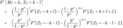
which coincides with {ZT = k + l}, due to our assumption l ≥ 0. Hence, the uniform distribution ℙ must assign the same probability to Ak,l and {ZT = k + l}, and we obtain our first formula. The second one follows by part one of this lemma:
Remark 5.48. Suppose that the random walk Z is defined even up to time T + 1; this can always be achieved by enlarging the probability space (Ω,F, ℙ). Then the probability in (5.32) can be rewritten as
Indeed, (5.34) is trivial in case T + k + l is not even; otherwise, we let j := (T + k + l)/2 and apply (5.31) to get

and the latter expression is equal to the right-hand side of (5.34).
◊
Formula (5.31) will change if we replace the uniform distribution ℙ by our martingale measure P∗, described in Theorem 5.39:

Let us now show how the reflection principle carries over to P∗.
Lemma 5.49 (Reflection principle for P∗). For all k ∈ ℕ and l ∈ ℕ0,

and
Proof. We show first that the density of P∗ with respect to ℙ is given by
Indeed, P∗ puts the weight
to each ω = (y1, . . . , yT) ∈ Ω which contains exactly k components with yi = +1. But for such an ω we have Z T(ω) = k − (T − k) = 2k − T, and our formula follows.
From the density formula (5.35), we get
Applying the reflection principle and using again the density formula, we see that the probability term on the right is equal to
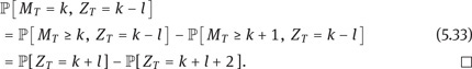
which gives the first identity. The proof of the second one is analogous. The second set of identities now follows as in (5.33).
Remark 5.50. If we assume once again that Z is defined up to time T + 1, then the arguments from the proof of Lemma 5.49 applied to (5.34) yield the alternative representation

Example 5.51 (Up-and-in call option). Consider an up-and-in call option with payoff

where B > S0 ∨ K denotes a given barrier, and where K > 0 is the strike price. Our aim is to compute the arbitrage-free price

The first expectation on the right can be computed explicitly in terms of the binomial distribution. Thus, it remains to compute the second expectation, whichwe denote by I. To this end, we may assume without loss of generality that B lies within the range of possible asset prices, i.e., there exists some k ∈ ℕ such that B = S0bk. Then, by Lemma 5.49,

where
Hence, we obtain the formula
Both expectations on the right now only involve the binomial distribution with parameters p∗ and T. They can be computed as in Example 5.42, and so we get the explicit formula

where n k is the largest integer n such that T −2n ≥ k and m k is the smallest integer m such that 2m > T + k.
◊
Example 5.52 (Up-and-out call option). Consider an up-and-out call option with payoff

where K > 0 is the strike price and B > S0 ∨ K is an upper barrier for the stock price. As in the preceding example, we assume that B = S0(1 + b)k for some k ∈ ℕ. Let
denote the corresponding “plain vanilla call”, whose arbitrage-free price is given by
Since ![]() we get from Example 5.51 that
we get from Example 5.51 that

where ![]() These expectations 0022can be computed as in Example 5.51.
These expectations 0022can be computed as in Example 5.51.
◊
Exercise 5.6.1. Derive a formula for the arbitrage-free price of a down-and-in put option with payoff

where K > 0 is the strike price and B < S0 is a lower barrier for the stock price. Then compute the price of the option for the following specific parameter values:
◊
In the following example, we compute the price of a lookback put option.
Example 5.53 (Lookback put option). A lookback put option corresponds to the contingent claim
see Example 5.23. In the CRR model, the discounted arbitrage-free price of ![]() is given by
is given by
The expectation of the maximum can be computed as
the formula (5.36) yields

Thus, we arrive at the expression

As before, one can give explicit formulas for the expectations occurring on the right-hand side.
◊
Exercise 5.6.2. Derive a formula for the price of a lookback call option with payoff
◊
5.7Convergence to the Black–Scholes price
In practice, a huge number of trading periods may occur between the current time t = 0 and the maturity T of a European contingent claim. Thus, the computation of option prices in terms of some martingale measure may become rather elaborate. On the other hand, one can hope that the pricing formulas in discrete time converge to a transparent limit as the number of intermediate trading periods grows larger and larger. In this section, we will formulate conditions under which such a convergence occurs.
Throughout this section, T will not denote the number of trading periods in a fixed discrete-time market model but rather a physical date. The time interval [0, T] will be divided into N equidistant time steps ![]() and the date
and the date ![]() will correspond to the kth trading period of an arbitrage-free market model. For simplicity, we will assume that each market model contains a riskless bond and just one risky asset. In the Nth approximation, the risky asset will be denoted by S(N), and the riskless bond will be defined by a constant interest rate rN > −1.
will correspond to the kth trading period of an arbitrage-free market model. For simplicity, we will assume that each market model contains a riskless bond and just one risky asset. In the Nth approximation, the risky asset will be denoted by S(N), and the riskless bond will be defined by a constant interest rate rN > −1.
The question is whether the prices of contingent claims in the approximating market models converge as N tends to infinity. Since the terminal values of the riskless bonds should converge, we assume that
where r is a finite constant. This condition is in fact equivalent to the following one:
Let us now consider the risky assets. We assume that the initial prices ![]() do not depend on
do not depend on ![]() for some constant S0 > 0. The prices
for some constant S0 > 0. The prices ![]() are random variables on some probability space
are random variables on some probability space ![]() where
where ![]() is a risk-neutral measure for each approximating market model, i.e., the discounted price process
is a risk-neutral measure for each approximating market model, i.e., the discounted price process
is a ![]() with respect to the filtration
with respect to the filtration ![]() Our remaining conditions will be stated in terms of the returns
Our remaining conditions will be stated in terms of the returns
First, we assume that, for each N, the random variables ![]() are independent under
are independent under ![]() and satisfy
and satisfy
for constants αN and βN such that
Second, we assume that the variances varN ![]() under
under ![]() are such that
are such that
The following result can be regarded as a multiplicative version of the central limit theorem.
Theorem 5.54. Under the above assumptions, the distributions of ![]() under
under ![]() converge weakly to the log-normal distribution with parameters log
converge weakly to the log-normal distribution with parameters log ![]() i.e., to the distribution of
i.e., to the distribution of
where WT has a centered normal law N (0, T) with variance T.
Proof. We may assume without loss of generality that S0 = 1. Consider the Taylor expansion
where the remainder term ρ is such that
and where δ(α, β) → 0 for α, β → 0. Applied to
this yields
Since ![]() is a martingale measure, we have
is a martingale measure, we have ![]() and it follows that
and it follows that
In particular, ΔN → 0 in probability, and the corresponding laws converge weakly to the Dirac measure δ0. Slutsky’s theorem, as stated in Appendix A.6, asserts that it suffices to show that the distributions of
converge weakly to the normal law ![]() To this end, we will check that the conditions of the central limit theorem in the form of Theorem A.41 are satisfied.
To this end, we will check that the conditions of the central limit theorem in the form of Theorem A.41 are satisfied.
Note that
for γN := |αN|∨ |βN|, and that
Finally,
since for p > 2
Thus, the conditions of Theorem A.41 are satisfied.
Remark 5.55. The assumption of independent returns in Theorem 5.54 can be relaxed. Instead of Theorem A.41, we can apply a central limit theorem for martingales under suitable assumptions on the behavior of the conditional variances
for details see, e.g., Section 9.3 of [57].
◊
Example 5.56. Suppose the approximating model in the Nth stage is a CRR model with interest rate
and with returns ![]() which can take the two possible values aN and bN; see Section 5.5. We assume that
which can take the two possible values aN and bN; see Section 5.5. We assume that
for some given σ > 0. Since
we have aN < rN < bN for large enough N. Theorem 5.39 yields that the Nth model is arbitrage-free and admits a unique equivalent martingale measure ![]() The measure
The measure ![]() is characterized by
is characterized by
and we obtain from (5.39) that
Moreover, ![]() and we get
and we get
as N ↑ ∞. Hence, the assumptions of Theorem 5.54 are satisfied.
◊
Let us consider a derivative which is defined in terms of a function f ≥ 0 of the risky asset’s terminal value. In each approximating model, this corresponds to a contingent claim
Corollary 5.57. If f is bounded and continuous, the arbitrage-free prices of ![]() calculated under
calculated under ![]() converge to a discounted expectation with respect to a log-normal distribution, which is often called the Black–Scholes price. More precisely,
converge to a discounted expectation with respect to a log-normal distribution, which is often called the Black–Scholes price. More precisely,

where ST has the form (5.37) under P∗.
This convergence result applies in particular to the choice f (x) = (K − x)+ corresponding to a European put option with strike K. Since the put-call parity
holds for each N and in the limit N ↑ ∞, the convergence (5.40) is also true for a European call option with the unbounded payoff profile f (x) = (x − K)+.
Example 5.58 (Black–Scholes formula for the price of a call option). The limit of the arbitrage-free prices of ![]() is given by v(S0, T), where
is given by v(S0, T), where
The integrand on the right vanishes for
Let us also define
and let us denote by ![]() dy the distribution function of the standard normal distribution. Then
dy the distribution function of the standard normal distribution. Then

Figure 5.5: The Black–Scholes price v(x, t) of a European call option (ST − K)+ plotted as a function of the initial spot price x = S0 and the time to maturity t.
and we arrive at the Black–Scholes formula for the price of a European call option with strike K and maturity T:
See Figure 5.5 for the plot of the function v(x, t).
◊
Remark 5.59. For fixed x and T, the Black–Scholes price of a European call option increases to the upper arbitrage bound x as σ ↑ ∞. In the limit σ ↓ 0, we obtain the lower arbitrage bound (x − e−rTK)+; see Remark 1.37.
◊
The following proposition gives a criterion for the convergence (5.40) in case f is not necessarily bounded and continuous. It applies in particular to f (x) = (x − K)+, and so we get an alternative proof for the convergence of call option prices to the Black–Scholes price.
Proposition 5.60. Let f : (0,∞) → ℝ be measurable, continuous a.e., and such that |f (x)| ≤ c (1 + x)q for some c ≥ 0 and 0 ≤ q < 2. Then
where ST has the form (5.37) under P∗.
Proof. Let us note first that by the Taylor expansion (5.38)

for a finite constant ![]() . Thus,
. Thus,
With this property established, the assertion follows immediately from Theorem 5.54 and the Corollaries A.49 and A.50, but we also give the following more elementary proof. To this end, we may assume that q > 0, and we define p := 2/q > 1. Then
and the assertion follows from Lemma 5.61 below.
Lemma 5.61. Suppose (μN)N∈N is a sequence of probability measures on ℝ converging weakly to μ. If f is a measurable and μ-a.e. continuous function on ℝ such that
then
Proof. We may assume without loss of generality that f ≥ 0. Then fk := f ∧ k is a bounded and μ-a.e. continuous function for each k > 0. Clearly,

Figure 5.6: The Delta Δ(x, t) of the Black–Scholes price of a European call option.
Due to part (e) of the portmanteau theorem in the form of Theorem A.43, the first ∫ integral on the right converges to fk dμ as N ↑ ∞. Let us consider the second term on the right:
uniformly in N. Hence,
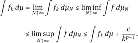
Letting k ↑ ∞, we have ![]() and convergence follows.
and convergence follows.
Let us now continue the discussion of the Black–Scholes price of a European call option where f (x) = (x − K)+. We are particularly interested how it depends on the various model parameters. The dependence on the spot price S0 = x can be analyzed via the x-derivatives of the function v(t, x) appearing in the Black–Scholes formula (5.41). The first derivative
is called the option’s Delta; see Figure 5.6. In analogy to the formula for the hedging strategy in the binomial model obtained in Proposition 5.44, Δ(x, t) determines the

Figure 5.7: The option’s Gamma Γ(x, t).
“Delta hedging portfolio” needed for a replication of the call option in continuous time, as explained in (5.51) below.
The Gamma of the call option is given by
see Figure 5.7. Here ![]() stands as usual for the density of the standard normal distribution. Large Gamma values occur in regions where the Delta changes rapidly, corresponding to the need for frequent readjustments of the Delta hedging portfolio. Note that Γ is always strictly positive. It follows that v(x, t) is a strictly convex function of its first argument.
stands as usual for the density of the standard normal distribution. Large Gamma values occur in regions where the Delta changes rapidly, corresponding to the need for frequent readjustments of the Delta hedging portfolio. Note that Γ is always strictly positive. It follows that v(x, t) is a strictly convex function of its first argument.
Exercise 5.7.1. Prove the formulas (5.42) and (5.43) for Delta and Gamma of a European call option.
◊
Remark 5.62. On the one hand, 0 ≤ Δ(x, t) ≤ 1 implies that
Thus, the total change of the option values is always less than a corresponding change in the asset prices. On the other hand, the strict convexity of ![]() together with (A.5) yields that for t > 0 and z > y
together with (A.5) yields that for t > 0 and z > y

Figure 5.8: The Theta Θ(x, t).
and hence
Similarly, one obtains
for x < y. Thus, the relative change of option prices is larger in absolute value than the relative change of asset values. This fact can be interpreted as the leverage effect for call options; see also Example 1.43.
◊
Another important parameter is the Theta
see Figure 5.8. The fact Θ > 0 corresponds to our general observation, made in Example 5.35, that arbitrage-free prices of European call options are typically increasing functions of the maturity.
Exercise 5.7.2. Prove the formula (5.44) for the Theta of a European call option. Then show that the parameters Δ, Γ, and Θ are related by the equation
◊
Equation (5.45) implies that, for (x, t) ∈ (0,∞)×(0,∞), the function v solves the partial differential equation
often called the Black–Scholes equation. Since
v(x, t) is a solution of the Cauchy problem defined via (5.46) and (5.47). This fact is not limited to call options, it remains valid for all reasonable payoff profiles f .
Proposition 5.63. Let f be a continuous function on (0,∞) such that |f (x)| ≤ c(1 + x)p for some c, p ≥ 0, and define
where St = x exp(σWt + rt − σ2t/2) and Wt has law N (0, t) under P∗. Then u solves the Cauchy problem defined by the Black–Scholes equation (5.46) and the initial condition limt↓0 u(x, t) = f (x), locally uniformly in x.
The proof of Proposition 5.63 is the content of the next exercise.
Exercise 5.7.3. In the context Proposition 5.63, use the formula (2.27) for the density of a log-normally distributed random variable to show that
where ![]() Then verify the validity of (5.46) by differentiating under the integral. Use the bound |f (x)| ≤ c(1 + x)p for some c, p ≥ 0 to justify the interchange of differentiation and integration and to verify the initial condition limt↓0 u(x, t) = f (x).
Then verify the validity of (5.46) by differentiating under the integral. Use the bound |f (x)| ≤ c(1 + x)p for some c, p ≥ 0 to justify the interchange of differentiation and integration and to verify the initial condition limt↓0 u(x, t) = f (x).
◊
Recall that the Black–Scholes price v(S0, T) was obtained as the expectation of the discounted payoff e−rT (ST − K)+ under the measure P∗. Thus, at a first glance, it may

Figure 5.9: The Rho ϱ(x, t) of a call option.
come as a surprise that the Rho of the option,
is strictly positive, i.e., the price is increasing in r; see Figure 5.9. Note, however, that the measure P∗ depends itself on the interest rate r, since E ∗[ e−rTST ] = S0. In a simple one-period model, we have already seen this effect in Example 1.43.
The parameter σ is called the volatility. As we have seen, the Black–Scholes price of a European call option is an increasing function of the volatility, and this is reflected in the strict positivity of
see Figure 5.10. The function V is often called the Vega of the call option price, and the functions Δ, Γ, Θ, ϱ, and V are usually called the Greeks (although “vega” does not correspond to a letter of the Greek alphabet).
Exercise 5.7.4. Prove the respective formulas (5.48) and (5.49) for Rho and Vega of a European call option. Then derive formulas for the option’s Vanna,
and the option’s Volga, which is also called Vomma,
◊
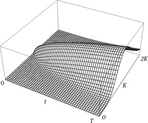
Figure 5.10: The Vega V (x, t).
Let us conclude this section with some informal comments on the dynamic picture in continuous time behind the convergence result in Theorem 5.54 and the pricing formulas in Example 5.58 and Proposition 5.60. The constant r is viewed as the interest rate of a riskfree savings account
The prices of the risky asset in each discrete-time model are considered as a continuous process ![]() defined as
defined as ![]() at the dates
at the dates ![]() and by linear interpolation in between. Theorem 5.54 shows that the distributions of
and by linear interpolation in between. Theorem 5.54 shows that the distributions of![]() converge for each fixed t weakly to the distribution of
converge for each fixed t weakly to the distribution of
where Wt has a centered normal distribution with variance t. In fact, one can prove convergence in the much stronger sense of a functional central limit theorem: The laws of the processes ![]() considered as C[0, T]-valued random variables on
considered as C[0, T]-valued random variables on ![]() converge weakly to the law of a geometric Brownian motion S = (St)0≤t≤T, where each St is of the form (5.50), and where the process W = (Wt)0≤t≤T is a standard Brownian motion or Wiener process. A Wiener process is characterized by the following properties:
converge weakly to the law of a geometric Brownian motion S = (St)0≤t≤T, where each St is of the form (5.50), and where the process W = (Wt)0≤t≤T is a standard Brownian motion or Wiener process. A Wiener process is characterized by the following properties:
–W0 = 0 almost surely,
–![]() is continuous,
is continuous,
–for each sequence 0 = t0 < t1 < ·· · < tn = T, the increments
are independent and have normal distributions N (0, ti − ti−1);
see, e.g., [177]. This multiplicative version of a functional central limit theorem follows as above if we replace the classical central limit theorem by Donsker’s invariance principle; for details see, e.g., [101]. Sample paths of Brownian motion and geometric Brownian motion can be found in Figures 5.11 and 5.12.

Figure 5.11: A sample path of Brownian motion.
Geometric Brownian motion is the classical reference model in continuous-time mathematical finance. In order to describe the model more explicitly, we denote by W = (Wt)0≤t≤T the coordinate process on the canonical path space Ω = C [0, T], defined by Wt(ω) = ω(t), and furthermore by (Ft)0≤t≤T the filtration given by Ft = σ(Ws; s ≤ t). There is exactly one probability measure ℙ on (Ω,FT) such that W is a Wiener process under ℙ, and it is called the Wiener measure. Let us now model the price process of a risky asset as a geometric Brownian motion S defined by (5.50). The discounted price process
is a martingale under ℙ, since
for 0 ≤ s ≤ t ≤ T. In fact, ℙ is the only probability measure equivalent to ℙ with that property.
As in discrete time, uniqueness of the equivalent martingale measure implies completeness of the model. Let us sketch the construction of the replicating strategy for a given European option with reasonable payoff profile f (ST), for example a call

Figure 5.12: A sample path of geometric Brownian motion.
option with strike K. At time t the price of the asset is S t(ω), the remaining time to maturity is T − t, and the discounted price of the option is given by
where u is the function defined in Proposition 5.63. The process V = (Vt)0≤t≤T can be viewed as the value process of the trading strategy ![]() = (ξ0, ξ) defined by
= (ξ0, ξ) defined by
where Δ = ∂u/∂x is the option’s Delta. Indeed, if we view ξ as the number of shares in the risky asset S and ξ0 as the number of shares in the riskfree savings account ![]() then the value of the resulting portfolio t0in units of the numéraire is given by
then the value of the resulting portfolio t0in units of the numéraire is given by
The strategy replicates the option since
due to Proposition 5.63. Moreover, its initial cost is given by the Black–Scholes price
It remains to show that the strategy is self-financing in the sense that changes in the portfolio value are only due to price changes in the underlying assets and do not require any additional capital. To this end, we use Itô’s formula
for a smooth function F, see, e.g., [177] or, for a strictly pathwise approach, [121]. Applied to the function F (x, t) = exp(σx + rt − σ2t/2), it shows that the price process S satisfies the stochastic differential equation
Thus, the infinitesimal return dSt/St is the sum of the safe return r dt and an additional noise term with zero expectation under P∗. The strength of the noise is measured by the volatility parameter σ. Similarly, we obtain
Applying Itô’s formula to the function
and using (5.52), we obtain
The Black–Scholes partial differential equation (5.46) shows that the term in parenthesis is equal to −rSt∂u/∂x, and we obtain from (5.53) that
More precisely,
where the integral with respect to X is defined as an Itô integral, i.e., as the limit of nonanticipating Riemann sums
along an increasing sequence (Dn) of partitions of the interval [0, T]; see, e.g., [121]. Thus, the Itô integral can be interpreted in financial terms as the cumulative net gain generated by dynamic hedging in the discounted risky asset as described by the hedging strategy ξ. This fact is an analogue of property (c) in Proposition 5.7, and in this sense ξ = (ξ0, ξ) is a self-financing trading strategy in continuous time. Similarly, we obtain the following continuous-time analogue of (5.5), which describes the undiscounted value of the portfolio as a result of dynamic trading both in the undiscounted risky asset and the riskfree asset:
Perfect replication also works for exotic options C (S) defined by reasonable functionals C on the path space C [0, T], due to a general representation theorem for such functionals as Itô integrals of the underlying Brownian motion W or, via (5.53), of the process X. Weak convergence on path space implies, in analogy to Proposition 5.63, that the arbitrage-free prices of the options C(S(N)), computed as discounted expectations under the measure ![]() converge to the discounted expectation
converge to the discounted expectation
under the Wiener measure ℙ.
On the other hand, the discussion in Section 5.6 suggests that the prices of certain exotic contingent claims, such as barrier options, can be computed in closed form as the Black–Scholes price for some corresponding payoff profile of the form f (ST). This is illustrated by the following example, where the price of an up-and-in call is computed in terms of the distribution of the terminal stock price under the equivalent martingale measure.
Example 5.64 (Black–Scholes price of an up-and-in call option). Consider an up-and-in call option

where B > S0 ∨ K denotes a given barrier, and where K > 0 is the strike price. As approximating models we choose the CRR models of Example 5.56. That is, we have interest rates
and parameters aN and b N defined by
for some given σ > 0. Applying the formula obtained in Example 5.51 yields

where
is the smallest integer k such that ![]() and
and
Then we have
Since f (x) = (x − K)+![]() {x≥B} is continuous a.e., we obtain
{x≥B} is continuous a.e., we obtain
due to Proposition 5.60. Combining the preceding argument with the fact that
also gives the convergence of the second expectation:
Next we note that for constants c, d > 0
due to l’Hôpital’s rule. From this fact, one deduces that
Thus, we may conclude that the arbitrage-free prices
in the Nth approximating model converge to
The expectations occurring in this formula are integrals with respect to a log-normal distribution and can be explicitly computed as in Example 5.58. Moreover, our limit is in fact equal to the Black–Scholes price of the up-and-in call option: The functional ![]() is continuous in each path in C [0, T] whose maximum is different from the value B, and one can show that these paths have full measure for the law of S under ℙ. Hence,
is continuous in each path in C [0, T] whose maximum is different from the value B, and one can show that these paths have full measure for the law of S under ℙ. Hence, ![]() is continuous ℙ ◦ S−1-a.e., and the functional version of Proposition 5.60 yields
is continuous ℙ ◦ S−1-a.e., and the functional version of Proposition 5.60 yields
so that our limiting price must coincide with the discounted expectation on the right.
◊
Remark 5.65. Let us assume, more generally, that the price process S is defined by
for some α ∈ ℝ. Applying Itô’s formula as in (5.52), we see that S is governed by the stochastic differential equation
with ![]() The discounted price process is given by
The discounted price process is given by
with ![]() for λ = (b − r)/σ. The process W∗ is a Wiener process under the measure P∗ ≈ ℙ defined by the density
for λ = (b − r)/σ. The process W∗ is a Wiener process under the measure P∗ ≈ ℙ defined by the density
In fact, P∗ is the unique equivalent martingale measure for X. We can now repeat the arguments above to conclude that the cost of perfect replication for a contingent claim C(S) is given by
◊
Even in the context of simple diffusion models such as geometric Brownian motion, however, completeness is lost as soon as the future behavior of the volatility parameter σ is unknown. If, for instance, volatility itself is modeled as a stochastic process, we are facing incompleteness. Thus, the problems of pricing and hedging in discrete-time incomplete markets as discussed in this book reappear in continuous time. Other versions of the invariance principle may lead to other classes of continuous-time models with discontinuous paths, for instance to geometric Poisson or Lévy processes. Discontinuity of paths is another important source of incompleteness. In fact, this has already been illustrated in this book, since discrete-time models can be regarded as stochastic processes in continuous time, where jumps occur at predictable dates.