3.3.4 Methods to process missing value attributes in DFDT

Search in book...
Toggle Font Controls
Create new playlist

Name your new playlist

Playlist description (optional)
Sign In

Email address

Password

Forgot Password?

or

Continue with Facebook

Continue with Google
Sign Up

Full Name

Email address

Confirm Email Address

Password

or

Continue with Facebook

Continue with Google

${[({\overset{↼}{v}}_{1}, {\overset{⇀}{v}}_{1}), ({\overset{↼}{v}}_{2}, {\overset{⇀}{v}}_{2})), [({\overset{↼}{v}}_{2}, {\overset{⇀}{v}}_{2}), ({\overset{↼}{v}}_{3}, {\overset{⇀}{v}}_{3})), \dots, [({\overset{↼}{v}}_{k - 1}, {\overset{⇀}{v}}_{k - 1}), ({\overset{↼}{v}}_{k}, {\overset{⇀}{v}}_{k}))} .$ ${[({\overset{↼}{v}}_{1}, {\overset{⇀}{v}}_{1}), ({\overset{↼}{v}}_{2}, {\overset{⇀}{v}}_{2})), [({\overset{↼}{v}}_{2}, {\overset{⇀}{v}}_{2}), ({\overset{↼}{v}}_{3}, {\overset{⇀}{v}}_{3})), \dots, [({\overset{↼}{v}}_{k - 1}, {\overset{⇀}{v}}_{k - 1}), ({\overset{↼}{v}}_{k}, {\overset{⇀}{v}}_{k}))} .$

Each interval is replaced with a dynamic fuzzy number $(\overset{↼}{α}, \overset{⇀}{α}),$ $(\overset{↼}{α}, \overset{⇀}{α}),$ thus completing the discretization of $({\overset{↼}{A}}_{i}, {\overset{⇀}{A}}_{i}) .$ $({\overset{↼}{A}}_{i}, {\overset{⇀}{A}}_{i}) .$ A division of the range of $({\overset{↼}{A}}_{i}, {\overset{⇀}{A}}_{i})$ $({\overset{↼}{A}}_{i}, {\overset{⇀}{A}}_{i})$ is called a discretization scheme. If two discretization schemes have the same division, then the two discretization schemes are equivalent.

As $| (\overset{↼}{U}, \overset{⇀}{U}) | ≜ n,$ $| (\overset{↼}{U}, \overset{⇀}{U}) | ≜ n,$ we have $\max (| {\overset{\leftarrow}{V}}_{{\overset{\leftarrow}{A}}_{1}}, {\vec{V}}_{{\vec{A}}_{1}} |) = n .$ $\max (| {\overset{\leftarrow}{V}}_{{\overset{\leftarrow}{A}}_{1}}, {\vec{V}}_{{\vec{A}}_{1}} |) = n .$ This is because there can be multiple separation points for the same value interval, and the resulting discretization schemes are equivalent. Therefore, it is possible to specify that a separation point can only exist at a value interval, and the number of separation points may be 0, 1, 2, ..., n − 1. When the number of separation points is j, there are Cjn−−1 methods for setting the separation points. There are $\sum_{j = 0}^{n - 1} C_{n - 1}^{j}$ $\sum_{j = 0}^{n - 1} C_{n - 1}^{j}$ kinds of discretization schemes in which the attribute $({\overset{↼}{A}}_{i}, {\overset{⇀}{A}}_{i})$ $({\overset{↼}{A}}_{i}, {\overset{⇀}{A}}_{i})$ is not equivalent. If there are m numerical attributes in the instance set, the number of corresponding discretized sets is at most 2(n−1)m. If the given instance set is finite, regardless of which method has been used, the discretization has a limited range. That is, the discrete set of the instance set is a finite field.

Suppose the condition attribute of the instance set is $(\overset{↼}{c}, \overset{⇀}{c}) = {({\overset{↼}{A}}_{1}, {\overset{⇀}{A}}_{1}),$ $(\overset{↼}{c}, \overset{⇀}{c}) = {({\overset{↼}{A}}_{1}, {\overset{⇀}{A}}_{1}),$ $({\overset{↼}{A}}_{2}, {\overset{⇀}{A}}_{2}), ..., ({\overset{↼}{A}}_{n} {\overset{⇀}{A}}_{n})}$ $({\overset{↼}{A}}_{2}, {\overset{⇀}{A}}_{2}), ..., ({\overset{↼}{A}}_{n} {\overset{⇀}{A}}_{n})}$ and the range of attribute $({\overset{↼}{A}}_{i}, {\overset{⇀}{A}}_{i}) \in (\overset{↼}{c}, \overset{⇀}{c}) i s ({\overset{↼}{V}}_{{\overset{↼}{A}}_{1}}, {\overset{⇀}{V}}_{{\overset{⇀}{A}}_{1}}) .$ $({\overset{↼}{A}}_{i}, {\overset{⇀}{A}}_{i}) \in (\overset{↼}{c}, \overset{⇀}{c}) i s ({\overset{↼}{V}}_{{\overset{↼}{A}}_{1}}, {\overset{⇀}{V}}_{{\overset{⇀}{A}}_{1}}) .$ A discretization scheme for a single numerical attribute $({\overset{↼}{A}}_{i}, {\overset{⇀}{A}}_{i})$ $({\overset{↼}{A}}_{i}, {\overset{⇀}{A}}_{i})$ is a partition $({\overset{↼}{π}}_{i}, {\overset{⇀}{π}}_{i}) o f ({\overset{↼}{V}}_{\overset{↼}{A}}, {\overset{⇀}{V}}_{\overset{⇀}{A}}) .$ $({\overset{↼}{π}}_{i}, {\overset{⇀}{π}}_{i}) o f ({\overset{↼}{V}}_{\overset{↼}{A}}, {\overset{⇀}{V}}_{\overset{⇀}{A}}) .$

The instance set $(\overset{↼}{U}, \overset{⇀}{U})$ $(\overset{↼}{U}, \overset{⇀}{U})$ filtered by attributes is denoted as $({\overset{↼}{U}}_{N}, {\overset{⇀}{U}}_{N}) . ({\overset{↼}{A}}_{i}, {\overset{⇀}{A}}_{i})$ $({\overset{↼}{U}}_{N}, {\overset{⇀}{U}}_{N}) . ({\overset{↼}{A}}_{i}, {\overset{⇀}{A}}_{i})$ is the conditional attribute of $({\overset{↼}{U}}_{N}, {\overset{⇀}{U}}_{N}), and ({\overset{↼}{A}}_{i}, {\overset{⇀}{A}}_{i})$ $({\overset{↼}{U}}_{N}, {\overset{⇀}{U}}_{N}), and ({\overset{↼}{A}}_{i}, {\overset{⇀}{A}}_{i})$ is numerical. Thus, the discretization of $({\overset{↼}{U}}_{N}, {\overset{⇀}{U}}_{N})$ $({\overset{↼}{U}}_{N}, {\overset{⇀}{U}}_{N})$ has multiple attributes.

Suppose that $({\overset{↼}{π}}_{1}, {\overset{⇀}{π}}_{1}) = ({\overset{↼}{π}}_{1}^{1}, {\overset{⇀}{π}}_{1}^{1}), ({\overset{↼}{π}}_{2}^{1}, {\overset{⇀}{π}}_{2}^{1}), ..., ({\overset{↼}{π}}_{n}^{1}, {\overset{⇀}{π}}_{n}^{1})} and ({\overset{↼}{π}}_{2}, {\overset{⇀}{π}}_{2}) =$ $({\overset{↼}{π}}_{1}, {\overset{⇀}{π}}_{1}) = ({\overset{↼}{π}}_{1}^{1}, {\overset{⇀}{π}}_{1}^{1}), ({\overset{↼}{π}}_{2}^{1}, {\overset{⇀}{π}}_{2}^{1}), ..., ({\overset{↼}{π}}_{n}^{1}, {\overset{⇀}{π}}_{n}^{1})} and ({\overset{↼}{π}}_{2}, {\overset{⇀}{π}}_{2}) =$ $({\overset{↼}{π}}_{1}^{2}, {\overset{⇀}{π}}_{1}^{2}), ({\overset{↼}{π}}_{2}^{2}, {\overset{⇀}{π}}_{2}^{2}), ..., ({\overset{↼}{π}}_{2}^{2}, {\overset{⇀}{π}}_{n}^{2})}$ $({\overset{↼}{π}}_{1}^{2}, {\overset{⇀}{π}}_{1}^{2}), ({\overset{↼}{π}}_{2}^{2}, {\overset{⇀}{π}}_{2}^{2}), ..., ({\overset{↼}{π}}_{2}^{2}, {\overset{⇀}{π}}_{n}^{2})}$ are two discretization schemes for instance set $({\overset{↼}{U}}_{N}, {\overset{⇀}{U}}_{N}), where ({\overset{↼}{π}}_{i}^{1}, {\overset{⇀}{π}}_{i}^{1})$ $({\overset{↼}{U}}_{N}, {\overset{⇀}{U}}_{N}), where ({\overset{↼}{π}}_{i}^{1}, {\overset{⇀}{π}}_{i}^{1})$ is the discretization scheme for attribute $({\overset{↼}{A}}_{i}, {\overset{⇀}{A}}_{i})$ $({\overset{↼}{A}}_{i}, {\overset{⇀}{A}}_{i})$ in $({\overset{↼}{π}}_{1}, {\overset{⇀}{π}}_{1}) . ({\overset{↼}{π}}_{i}^{2}, {\overset{⇀}{π}}_{i}^{2})$ $({\overset{↼}{π}}_{1}, {\overset{⇀}{π}}_{1}) . ({\overset{↼}{π}}_{i}^{2}, {\overset{⇀}{π}}_{i}^{2})$ is the discretization scheme for attribute $({\overset{↼}{A}}_{j}, {\overset{⇀}{A}}_{j}) in ({\overset{↼}{π}}_{2}, {\overset{⇀}{π}}_{2}) .$ $({\overset{↼}{A}}_{j}, {\overset{⇀}{A}}_{j}) in ({\overset{↼}{π}}_{2}, {\overset{⇀}{π}}_{2}) .$

As $({\overset{↼}{π}}_{j}^{i}, {\overset{⇀}{π}}_{j}^{i})$ $({\overset{↼}{π}}_{j}^{i}, {\overset{⇀}{π}}_{j}^{i})$ is the discretization scheme for attribute $({\overset{↼}{A}}_{j}, {\overset{⇀}{A}}_{j}),$ $({\overset{↼}{A}}_{j}, {\overset{⇀}{A}}_{j}),$ the partial order relation in the discretization is defined as follows:

Discretization scheme $({\overset{↼}{π}}_{i}, {\overset{⇀}{π}}_{i}) \leq ({\overset{↼}{π}}_{j}, {\overset{⇀}{π}}_{j}) if and only if ({\overset{↼}{π}}_{k}^{i}, {\overset{⇀}{π}}_{k}^{i}) \leq ({\overset{↼}{π}}_{k}^{j}, {\overset{⇀}{π}}_{k}^{j})$ $({\overset{↼}{π}}_{i}, {\overset{⇀}{π}}_{i}) \leq ({\overset{↼}{π}}_{j}, {\overset{⇀}{π}}_{j}) if and only if ({\overset{↼}{π}}_{k}^{i}, {\overset{⇀}{π}}_{k}^{i}) \leq ({\overset{↼}{π}}_{k}^{j}, {\overset{⇀}{π}}_{k}^{j})$ (k = 1, 2, . . ., n) is satisfied for each attribute $({\overset{↼}{A}}_{k}, {\overset{⇀}{A}}_{k})$ $({\overset{↼}{A}}_{k}, {\overset{⇀}{A}}_{k})$ in instance set $({\overset{↼}{U}}_{N}, {\overset{⇀}{U}}_{N}),$ $({\overset{↼}{U}}_{N}, {\overset{⇀}{U}}_{N}),$ where $({\overset{↼}{π}}_{k}^{i}, {\overset{⇀}{π}}_{k}^{i})$ $({\overset{↼}{π}}_{k}^{i}, {\overset{⇀}{π}}_{k}^{i})$ is the division of $({\overset{↼}{V}}_{{\overset{↼}{A}}_{k}}, {\overset{⇀}{V}}_{{\overset{⇀}{A}}_{k}}) i n ({\overset{↼}{π}}_{i}, {\overset{⇀}{π}}_{i})$ $({\overset{↼}{V}}_{{\overset{↼}{A}}_{k}}, {\overset{⇀}{V}}_{{\overset{⇀}{A}}_{k}}) i n ({\overset{↼}{π}}_{i}, {\overset{⇀}{π}}_{i})$ . The relation ≤ defines the degree of discretization among the discretization schemes as a partial order relation.

$({\overset{↼}{π}}_{k}^{i}, {\overset{⇀}{π}}_{k}^{i}) \leq ({\overset{↼}{π}}_{k}^{j}, {\overset{⇀}{π}}_{k}^{j})$ $({\overset{↼}{π}}_{k}^{i}, {\overset{⇀}{π}}_{k}^{i}) \leq ({\overset{↼}{π}}_{k}^{j}, {\overset{⇀}{π}}_{k}^{j})$ indicates that $({\overset{↼}{π}}_{i}, {\overset{⇀}{π}}_{i})$ $({\overset{↼}{π}}_{i}, {\overset{⇀}{π}}_{i})$ divides the value of attribute $({\overset{↼}{A}}_{k}, {\overset{⇀}{A}}_{k})$ $({\overset{↼}{A}}_{k}, {\overset{⇀}{A}}_{k})$ into a range. Then, the division of the value of attribute $({\overset{↼}{A}}_{k}, {\overset{⇀}{A}}_{k})$ $({\overset{↼}{A}}_{k}, {\overset{⇀}{A}}_{k})$ must belong to the same range. Two or more adjacent segmentation intervals of the value of attribute $({\overset{↼}{A}}_{k}, {\overset{⇀}{A}}_{k})$ $({\overset{↼}{A}}_{k}, {\overset{⇀}{A}}_{k})$ are merged into one interval of attribute $({\overset{↼}{A}}_{k}, {\overset{⇀}{A}}_{k}) in ({\overset{↼}{π}}_{j}, {\overset{⇀}{π}}_{j}) . As ({\overset{↼}{π}}_{i}, {\overset{⇀}{π}}_{i}) \leq ({\overset{↼}{π}}_{j}, {\overset{⇀}{π}}_{j}), ({\overset{↼}{π}}_{i}, {\overset{⇀}{π}}_{i})$ $({\overset{↼}{A}}_{k}, {\overset{⇀}{A}}_{k}) in ({\overset{↼}{π}}_{j}, {\overset{⇀}{π}}_{j}) . As ({\overset{↼}{π}}_{i}, {\overset{⇀}{π}}_{i}) \leq ({\overset{↼}{π}}_{j}, {\overset{⇀}{π}}_{j}), ({\overset{↼}{π}}_{i}, {\overset{⇀}{π}}_{i})$ is the refinement of $({\overset{↼}{π}}_{j}, {\overset{⇀}{π}}_{j}) .$ $({\overset{↼}{π}}_{j}, {\overset{⇀}{π}}_{j}) .$

The intersection and union operations of the discretization scheme for instance set $({\overset{↼}{U}}_{N}, {\overset{⇀}{U}}_{N})$ $({\overset{↼}{U}}_{N}, {\overset{⇀}{U}}_{N})$ are

$\begin{array}{l} ({\overset{↼}{π}}_{i}, {\overset{⇀}{π}}_{i}) \cap ({\overset{↼}{π}}_{j}, {\overset{⇀}{π}}_{j}) = {({\overset{↼}{π}}_{1}^{i}, {\overset{↼}{π}}_{1}^{i}) \land ({\overset{↼}{π}}_{1}^{j}, {\overset{↼}{π}}_{1}^{j}), ({\overset{↼}{π}}_{2}^{i}, {\overset{↼}{π}}_{2}^{i}) \land ({\overset{↼}{π}}_{2}^{j}, {\overset{↼}{π}}_{2}^{j}), \\ \dots, ({\overset{↼}{π}}_{n}^{i}, {\overset{↼}{π}}_{n}^{i}) \land ({\overset{↼}{π}}_{n}^{j}, {\overset{↼}{π}}_{n}^{j})} \end{array}$ $\begin{array}{l} ({\overset{↼}{π}}_{i}, {\overset{⇀}{π}}_{i}) \cap ({\overset{↼}{π}}_{j}, {\overset{⇀}{π}}_{j}) = {({\overset{↼}{π}}_{1}^{i}, {\overset{↼}{π}}_{1}^{i}) \land ({\overset{↼}{π}}_{1}^{j}, {\overset{↼}{π}}_{1}^{j}), ({\overset{↼}{π}}_{2}^{i}, {\overset{↼}{π}}_{2}^{i}) \land ({\overset{↼}{π}}_{2}^{j}, {\overset{↼}{π}}_{2}^{j}), \\ \dots, ({\overset{↼}{π}}_{n}^{i}, {\overset{↼}{π}}_{n}^{i}) \land ({\overset{↼}{π}}_{n}^{j}, {\overset{↼}{π}}_{n}^{j})} \end{array}$

$\begin{array}{l} ({\overset{↼}{π}}_{i}, {\overset{⇀}{π}}_{i}) \cup ({\overset{↼}{π}}_{j}, {\overset{⇀}{π}}_{j}) = {({\overset{↼}{π}}_{1}^{i}, {\overset{↼}{π}}_{1}^{i}) \lor ({\overset{↼}{π}}_{1}^{j}, {\overset{↼}{π}}_{1}^{j}), ({\overset{↼}{π}}_{2}^{i}, {\overset{↼}{π}}_{2}^{i}) \lor ({\overset{↼}{π}}_{2}^{j}, {\overset{↼}{π}}_{2}^{j}), \\ \dots, ({\overset{↼}{π}}_{n}^{i}, {\overset{↼}{π}}_{n}^{i}) \lor ({\overset{↼}{π}}_{n}^{j}, {\overset{↼}{π}}_{n}^{j})} . \end{array}$ $\begin{array}{l} ({\overset{↼}{π}}_{i}, {\overset{⇀}{π}}_{i}) \cup ({\overset{↼}{π}}_{j}, {\overset{⇀}{π}}_{j}) = {({\overset{↼}{π}}_{1}^{i}, {\overset{↼}{π}}_{1}^{i}) \lor ({\overset{↼}{π}}_{1}^{j}, {\overset{↼}{π}}_{1}^{j}), ({\overset{↼}{π}}_{2}^{i}, {\overset{↼}{π}}_{2}^{i}) \lor ({\overset{↼}{π}}_{2}^{j}, {\overset{↼}{π}}_{2}^{j}), \\ \dots, ({\overset{↼}{π}}_{n}^{i}, {\overset{↼}{π}}_{n}^{i}) \lor ({\overset{↼}{π}}_{n}^{j}, {\overset{↼}{π}}_{n}^{j})} . \end{array}$

The partition of instance set $({\overset{↼}{U}}_{N}, {\overset{⇀}{U}}_{N})$ $({\overset{↼}{U}}_{N}, {\overset{⇀}{U}}_{N})$ divided by $({\overset{↼}{π}}_{i}, {\overset{⇀}{π}}_{i}) \cap ({\overset{↼}{π}}_{j}, {\overset{⇀}{π}}_{j})$ $({\overset{↼}{π}}_{i}, {\overset{⇀}{π}}_{i}) \cap ({\overset{↼}{π}}_{j}, {\overset{⇀}{π}}_{j})$ is the biggest partition that is smaller than that divided by $({\overset{↼}{π}}_{i}, {\overset{⇀}{π}}_{i}) and ({\overset{↼}{π}}_{j}, {\overset{⇀}{π}}_{j}), similarly, ({\overset{↼}{π}}_{i},)$ $({\overset{↼}{π}}_{i}, {\overset{⇀}{π}}_{i}) and ({\overset{↼}{π}}_{j}, {\overset{⇀}{π}}_{j}), similarly, ({\overset{↼}{π}}_{i},)$ . Similarly, ${\overset{⇀}{π}}_{i}) \cup ({\overset{↼}{π}}_{j}, {\overset{⇀}{π}}_{j})$ ${\overset{⇀}{π}}_{i}) \cup ({\overset{↼}{π}}_{j}, {\overset{⇀}{π}}_{j})$ ${\overset{⇀}{π}}_{i}) \cup ({\overset{↼}{π}}_{j}, {\overset{⇀}{π}}_{j})$ ${\overset{⇀}{π}}_{i}) \cup ({\overset{↼}{π}}_{j}, {\overset{⇀}{π}}_{j})$ is the smallest partition that is bigger than both $({\overset{↼}{π}}_{i}, {\overset{⇀}{π}}_{i}) and ({\overset{↼}{π}}_{j}, {\overset{⇀}{π}}_{j}) .$ $({\overset{↼}{π}}_{i}, {\overset{⇀}{π}}_{i}) and ({\overset{↼}{π}}_{j}, {\overset{⇀}{π}}_{j}) .$

Define the partial order ≤ and the intersection and union operations of the discretization scheme. Then, the lattice structure with the discretization scheme of the instance set as an element can be obtained. This is called the Dynamic Fuzzy Discrete Lattice [36].

Because all kinds of discretization schemes are elements of the Dynamic Fuzzy Discrete Lattice, the discretization of instance set $({\overset{↼}{U}}_{N}, {\overset{⇀}{U}}_{N})$ $({\overset{↼}{U}}_{N}, {\overset{⇀}{U}}_{N})$ is transformed into a search problem on the Dynamic Fuzzy Discrete Lattice. When attribute $({\overset{↼}{A}}_{i}, {\overset{⇀}{A}}_{i})$ $({\overset{↼}{A}}_{i}, {\overset{⇀}{A}}_{i})$ is discretized, there are many separation points in $({\overset{↼}{V}}_{{\overset{↼}{A}}_{1}}, {\overset{⇀}{V}}_{{\overset{⇀}{A}}_{1}}) .$ $({\overset{↼}{V}}_{{\overset{↼}{A}}_{1}}, {\overset{⇀}{V}}_{{\overset{⇀}{A}}_{1}}) .$ If there are some separation points that will not affect the discretization result after being deleted, these nodes are redundant separation points.

Definition 3.4 For attribute $({\overset{↼}{A}}_{i}, {\overset{⇀}{A}}_{i}),$ $({\overset{↼}{A}}_{i}, {\overset{⇀}{A}}_{i}),$ there is a set of separation points $(\overset{↼}{s}, \overset{⇀}{s}) =$ $(\overset{↼}{s}, \overset{⇀}{s}) =$ ${({\overset{↼}{s}}_{1}, {\overset{⇀}{s}}_{1}), ({\overset{↼}{s}}_{2}, {\overset{⇀}{s}}_{2}), ..., ({\overset{↼}{s}}_{k}, {\overset{⇀}{s}}_{k})} . if ({\overset{↼}{s}}_{i}, {\overset{⇀}{s}}_{i}) \in (\overset{↼}{s}, \overset{⇀}{s})$ ${({\overset{↼}{s}}_{1}, {\overset{⇀}{s}}_{1}), ({\overset{↼}{s}}_{2}, {\overset{⇀}{s}}_{2}), ..., ({\overset{↼}{s}}_{k}, {\overset{⇀}{s}}_{k})} . if ({\overset{↼}{s}}_{i}, {\overset{⇀}{s}}_{i}) \in (\overset{↼}{s}, \overset{⇀}{s})$ is deleted and its two separate intervals are merged, the attribute values in the two intervals are replaced by the same dynamic fuzzy number $(\overset{↼}{α}, \overset{⇀}{α}) .$ $(\overset{↼}{α}, \overset{⇀}{α}) .$ The resulting instance set is the same, and the separation point $({\overset{↼}{s}}_{i}, {\overset{⇀}{s}}_{i}) \in (\overset{↼}{s}, \overset{⇀}{s})$ $({\overset{↼}{s}}_{i}, {\overset{⇀}{s}}_{i}) \in (\overset{↼}{s}, \overset{⇀}{s})$ is called a redundant separation point.

Definition 3.5 The number of redundant separation points in a discretization scheme of attribute $({\overset{↼}{A}}_{i}, {\overset{⇀}{A}}_{i})$ $({\overset{↼}{A}}_{i}, {\overset{⇀}{A}}_{i})$ is called the separation point level.

Obviously, the higher the separation point level, the more corresponding redundant points exist for the discretization of this attribute.

The goal of the discretization of attributes is to keep the discretization results consistent and to minimize the number of redundant separation points [37]. The basic steps are as follows: calculate the separation point level of each attribute; sort attributes in ascending order of the separation point level; delete the redundant divider points one by one. The algorithm is described as:

(1)Find the separation point level for each discretization attribute and the set of separable points that can be removed.

(2)Each attribute is sorted in ascending order according to the separation point level, and a sequence of attributes is obtained.

(3)Each attribute in the attribute sequence is processed one after the other. If there is a redundant separation point at the i th attribute, merge the interval adjacent to this separation point and judge the consistency of the instance set. The number of redundant separation points for the i th attribute decreases by one, and the instance set is updated. Otherwise, the separation point is retained. Go to (3) and perform the next round of operations on redundant separation points.

(4)If there are no redundant separation points for each attribute in the attribute sequence, the algorithm ends and a discretized instance set is obtained.

It can be seen from the algorithm that the operation of deleting redundant separation points enhances the discretization scheme, and a sequence of discretization schemes with decreasing separation points is obtained. The two adjacent discretization schemes in the sequence satisfy the partial order relation ≤. The last scheme in the sequence is the discretization scheme of instance set $({\overset{↼}{U}}_{N}, {\overset{⇀}{U}}_{N}) .$ $({\overset{↼}{U}}_{N}, {\overset{⇀}{U}}_{N}) .$

In the discretization based on the Dynamic Fuzzy Partition Lattice, the first consideration is the consistency of the instance set. The consistency can limit the degree of approximation to the original set, avoiding the conflict of data caused by discretization based on information entropy. By operating according to the value of the attributes without artificially terminating the algorithm, the impact of human factors in the discretization of the instance set is reduced.

3.3.4Methods to process missing value attributes in DFDT

1. Reasons for data loss

Missing attribute values are a frequent and inevitable occurrence in datasets that reflect practical problems. Therefore, in most cases, the information system is incomplete, or there is a certain degree of incompleteness. The reasons for missing data are multifaceted [33, 42] and concluded as follows:

(1)Some information is temporarily unavailable. For example, in medical databases, not all of the clinical test results of all patients can be given within a certain time, resulting in some of the attribute values being empty. Furthermore, the response to certain questions depends on the answers to other questions in application form data.

(2)Some information is missing. This may be because the data are considered unimportant when they are input, simply forgotten, or some misunderstanding occurs. Additionally, it is possible that the data acquisition equipment, storage media, or transmission media have failed, or some human factor has resulted in the data loss.

(3)One or more properties of some object are not available. In other words, the attribute value does not exist for this object. Examples include an unmarried person asked for their spouse’s name or a child’s fixed income status.

(4)Some information is (considered) unimportant.

(5)The cost of obtaining this information is too high.

(6)Real-time performance requirements of the system are high, meaning that judgments or decisions must be made before such information can be obtained.

2. Importance and complexity of processing missing values

Data loss is a complex problem in many fields of research. The existence of null values has the following effects [40]: First, the system has lost some useful information. Second, the uncertainty of the system increases, as deterministic elements in the system are more difficult to quantify. Finally, data that contain null values will lead to confusion in the learning process, resulting in unreliable output.

Decision tree algorithms are committed to avoiding the problem of overfitting the training set. This feature makes it difficult to deal with incomplete data. Therefore, missing values need to be handled through specialized methods such as filling to reduce the distance between the algorithms and reality.

3. Analysis and comparison of missing value processing methods

There are three main methods for dealing with incomplete instance sets:

A. Delete the tuple

That is, delete the instance that has missing information attribute values, leaving a complete set of instances. This method is simple, effective in cases where the instance includes multiple attribute missing values, and the number of deleted objects with missing values is very small compared to the whole set of instances. However, this approach has great limitations. It will result in wasted resources, as the information hidden in these instances will be discarded. If the set includes a small number of instances, deleting just a few objects could seriously affect the information objectivity and the correctness of the results. When the percentage of the value of each property changes significantly, performance becomes very poor. Thus, when a large percentage of missing data is available, particularly when missing data is not randomly distributed, this approach can lead to deviations in the data and erroneous conclusions [44].

B. Complete the data

This method completes the set of instances by filling in the missing values. The values used to fill in the missing data are usually based on statistical principles according to the distribution of the other objects in the dataset, e.g. average value of the remaining attributes. Table 3.7 lists some commonly used methods of filling in missing values.

C. Not handled

Create the decision tree directly based on the set of instances that contain missing values.

Tab. 3.7: Comparison of missing value filling methods [45–48].

4. Classification of missing values in DFDT

The missing attribute values should be divided into the following three cases and handled separately in DFDT:

(1)Attribute values that contribute no information to the classification;

(2)Attribute values that partly contribute information to the classification;

(3)Attribute values that play an important role in the classification, i.e. important sources of information.

An example is given below to illustrate how DFDT treats these three types of missing attribute values. Assume that the following attributes are present in the dataset that determines the incidence of influenza: name, gender, geography, age, onset time, temperature. We seek to identify those attribute and classification results that are not necessarily linked; i.e. for this category name, the attribute does not contribute any information. There are two types of treatment for such attributes:

(1) Delete this attribute directly from the dataset.

This approach is essentially the first method of dealing with incomplete data, but it also inherits the shortcomings of the delete tuple method.

(2) Conduct a type of discretization operation. For example, assign a dynamic fuzzy number to the name attribute of all instances (for instance, “name” = 0.5). The advantage of this approach is that it maintains the integrity of the dataset.

The time attribute contributes some information to the classification; e.g. from the “2005-10-10” value of the “onset time” property, we may infer that October is the high incidence period of influenza. We first simplify the attribute values and retain the useful information for classification. For the attributes that have been simplified, their values make a complete contribution to the classification; i.e. the contribution has increased from a partial contribution to an important contribution. When the simplified attribute value is missing, the same processing method as for important attributes is applied. The processing of important attributes is divided into techniques for the training instance set and the test set [37].

Processing methods for the training set:

(1)Ignore the instance that contains the missing value attribute.

(2)Assign values to the attribute using information from other instances. Assume that the attribute of instance A belonging to class C is unknown. Values are assigned to A according to the other instances belonging to class C.

(3)Obtain the attribute value using the decision tree method.

Assume that the training set S has a partially unknown value of attribute A. Select the instances that in which attribute A is known from S, and compose the subset S′ using these selected instances. Create a decision tree in set S′ by processing the original classification attribute as a general attribute. Let A be the classification attribute of S′, and generate the decision tree and rules that can be used to assign values to attribute A in set S− S′.

(4) Assign value “unknown” to the attribute.

These methods have advantages and disadvantages. Method (1), although simple, will inevitably lead to the loss of information and the destruction of information integrity. Method (3) is complicated and applies only to the case where relatively few attribute values are missing. Method (4) considers the value “unknown” as an attribute value in the dataset, which changes the domain of the value. Although method (2) may be affected by subjective factors, and the criterion for a correlation between instances is difficult to determine, it is known to be highly practical. Because of the obvious disadvantages of the other three methods, we use method (2) to deal with important missing value attributes in the training set in DFDT.

After processing the missing value attributes in the training set, we can create the decision tree. We should test the decision tree using the test instance set. When classifying instances of the test set, if the instance contains missing attribute values, the classification immediately becomes impossible because we do not know which branch this instance will go into in the decision tree. In this case, we need to deal with the missing attribute values in the test set. There are many ways to deal with missing attribute values in a test set, such as agent attribute segmentation (Breiman et al. 1984) [51], dynamic path generation (White 1987, Liu & White 1994) [52, 53] and the lazy decision tree method (Friedman et al. 1996) [54]. In DFDT, the action is similar to that taken for the training instance set: a value is assigned to the attribute using information from other instances.

3.4Pruning strategy of DFDT

3.4.1Reasons for pruning

After feature extraction and the processing of special features in the previous stage, we can now build the decision tree according to the training dataset. The decision tree is built on the basis of classifying the training data. Next, we classify the surplus instances in the instance space. At this point, we must determine whether the established decision tree achieves acceptable performance. For this, a validation process is needed. This may involve extra instances from the test set or the application of cross-validation. Here, we adopt algorithm C4.5 with cross-validation and conduct tests on several datasets from the UCI repository (further information can be found in Tab. 3.8). The test data are presented in Tab. 3.9.

From Tab. 3.9, it can be seen that if there is noise in the data or the number of training instances is too small to obtain typical samples, we will have problems in building the decision tree.

Tab. 3.8: Information of UCI dataset.

Tab. 3.9: Decision tree accuracy.

For a given assumption, if there are other assumptions that fit the training instances worse but fit the whole instance space better, we say that the assumption overfits the training instances.

Definition 3.6 Giving an assumption space H and an assumption h∈ H, if there is H such that the error rate of h is smaller than that of h′ in the training instances but the error rate of h′ is smaller across the whole set of instances, we say that h overfits the training instances.

What causes tree h to fit better than tree h′ on the training instances but achieve worse performance on the other instances? One reason is that there is random error or noise in the training instances. For example, we add a positive training instance in PlayTennis (Tab. 3.3), but it is wrongly labelled as negative:

Outlook = Sunny, Temperature = Hot, Humidity = Normal

Wind = Strong, PlayTennis = No

We build the decision tree from positive data using algorithm ID3 and generate the decision tree (Fig. 3.4). However, when adding the wrong instance, it generates a more complex structure (Fig. 3.6).

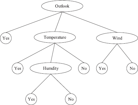
Certainly, h will fit the training instance set perfectly, whereas h′ will not. However, the new decision node is produced by fitting the noise in the training instances. We can conclude that h′ will achieve better performance than h in the data extracted from the same instance distribution.

From this example, we can see that random error or noise in the training instances will lead to overfitting. However, overfitting also occurs without noise, especially when fewer instances are associated.

To avoid a complex and huge decision tree caused by overfitting and too many branches, we apply a pruning process to the branches.

3.4.2Methods of pruning

There are several methods to prevent overfitting in learning a decision tree. These methods are divided into two classes.

Pre-pruning: Stop the growth of the tree before correctly classifying the training set completely. There are many different methods to determine when to stop the growth of the decision tree. Pre-pruning is a direct strategy that prevents overfitting during tree building. At the same time, there is no need for pre-pruning to generate the whole decision tree, leading to high efficiency, which makes it a suitable strategy for large-scale questions. However, there is a disadvantage. It is difficult to accurately identify when to stop the growth. That is, under the same standard, maybe the current extension is unable to meet the demand, but a further extension will. Thus, if the algorithm terminates too early, useful information will be missed.

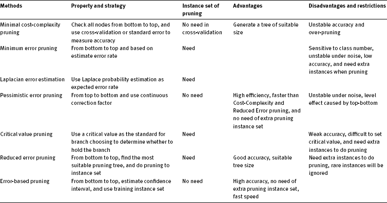
Post-pruning: Overfitting is permitted, and then pruning is applied. Post-pruning, as proposed by Breiman et al. (1984), has been widely discussed and can achieve great success in applications such as Cost-Complexity Pruning, Minimum Error Pruning, Pessimistic Error Pruning, Critical Value Pruning, Reduced Error Pruning, and Error-Based Pruning (EBP). Table 3.10 gives a summary of several decision tree pruning methods.

3.4.3DFDT pruning strategy

Unlike pre-pruning, which is suitable for large-scale problems, post-pruning is known to be successful in practice. In the preliminary stage of DFDT, the scale of the dataset is not too large. We prefer not to interpose when building DFDT, so that we obtain an unpruned original decision tree. Then, we can determine whether DFDT is good or bad from the classification error rate of the original decision tree. Thus, post-pruning is much more suitable for DFDT. There is no need for EBP to use an extra pruning instances set. Through the process of pruning, DFDT can attain low complexity under the premise of the original predictive power.

EBP checks each subtree from bottom to top, computes the estimated error rate for each subtree, and returns it as the error rate of a leaf node. If a branch is unable to reduce the error rate, then it will be pruned. In other words, if the error rate of the subtree is larger than that of the leaf node, the subtree is returned to a leaf node.

The estimated error rate of a leaf node is given by

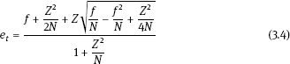
where N is the number of instances of the leaf node, f = E/ N is the classification error rate of the node, and E is the number of erroneous classifications. When the reliability is 25%, Z is 0.69.

The estimated error rate of a subtree is given by

where N is the number of instances in the root node number of subtree T, and Ni is the number of instances of T in the i th node.

Tab. 3.10: Comparison of different pruning methods. [9, 10, 48, 49]

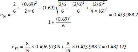
Next, we use an example to explain the pruning process. The system adopts a bottom-to-top strategy to check all subtrees in the decision tree and compute et and eT. If et < eT, then the pruning is conducted as shown in Fig. 3.7.

First, we find a subtree and compute et4 using (3.4). That is, we return the error rate to that of the leaf node. Next, we use (3.5) to compute eT4, saving the estimated error rate of the subtree. At this point, eT4 (= 0.487 ) (=0.591 ); thus, saving is smaller than et4 T4 can reduce the error rate, so we do not prune T4. on the procedure is repeated for all subtrees. When we have checked the root node, the whole tree has been pruned.

\begin{array}{l} e_{t 4} = \frac{\frac{7}{4} + \frac{{(0.69)}^{2}}{2 \times 14} + (1.69) \sqrt{\frac{7 / 14}{14} - \frac{{(7 / 14)}^{2}}{14} + \frac{{(7 / 14)}^{2}}{4 \times {(14)}^{2}}}}{1 + \frac{{(0.69)}^{2}}{14}} = 0.590 676 \\ e_{t 5} = \frac{\frac{3}{8} + \frac{{(0.69)}^{2}}{2 \times 8} + (1.69) \sqrt{\frac{3 / 8}{8} - \frac{{(3 / 8)}^{2}}{8} + \frac{{(3 / 8)}^{2}}{4 \times {(8)}^{2}}}}{1 + \frac{{(0.69)}^{2}}{8}} = 0.496 973 6 \end{array}

$\begin{array}{l} e_{t 4} = \frac{\frac{7}{4} + \frac{{(0.69)}^{2}}{2 \times 14} + (1.69) \sqrt{\frac{7 / 14}{14} - \frac{{(7 / 14)}^{2}}{14} + \frac{{(7 / 14)}^{2}}{4 \times {(14)}^{2}}}}{1 + \frac{{(0.69)}^{2}}{14}} = 0.590 676 \\ e_{t 5} = \frac{\frac{3}{8} + \frac{{(0.69)}^{2}}{2 \times 8} + (1.69) \sqrt{\frac{3 / 8}{8} - \frac{{(3 / 8)}^{2}}{8} + \frac{{(3 / 8)}^{2}}{4 \times {(8)}^{2}}}}{1 + \frac{{(0.69)}^{2}}{8}} = 0.496 973 6 \end{array}$

Fig. 3.7: Pruning of decision tree.

While pruning, EBP deletes subtrees and then grafts them to the father node of the deleted tree.

3.5Application

..................Content has been hidden....................

You can't read the all page of ebook, please click here login for view all page.

Table of Contents for 3.3.4 Methods to process missing value attributes in DFDT

Create new playlist

Sign In