4.5.3 DF concept rule extraction and matching algorithm

Search in book...
Toggle Font Controls
Create new playlist

Name your new playlist

Playlist description (optional)
Sign In

Email address

Password

Forgot Password?

or

Continue with Facebook

Continue with Google
Sign Up

Full Name

Email address

Confirm Email Address

Password

or

Continue with Facebook

Continue with Google

The intersection and union operations of the discretization scheme of set $({\overset{↼}{U}}_{N}, {\overset{⇀}{U}}_{N})$ $({\overset{↼}{U}}_{N}, {\overset{⇀}{U}}_{N})$ are

$\begin{array}{l} ({\overset{\leftarrow}{π}}_{i}, {\overset{⇀}{π}}_{i}) \cap ({\overset{\leftarrow}{π}}_{j}, {\overset{⇀}{π}}_{j}) = {(π_{1}^{i}, π_{1}^{i}) \land (π_{1}^{i}, π_{1}^{j}), (π_{2}^{i}, π_{2}^{j}) \land (π_{2}^{j}, π_{2}^{j}), \dots, (π_{n}^{i}, π_{n}^{j}) \land (π_{n}^{i}, π_{n}^{j})} \\ ({\overset{\leftarrow}{π}}_{i}, {\overset{⇀}{π}}_{i}) \cup ({\overset{\leftarrow}{π}}_{j}, {\overset{⇀}{π}}_{j}) = {(π_{1}^{i}, π_{1}^{i}) \lor (π_{1}^{i}, π_{1}^{j}), (π_{2}^{i}, π_{2}^{j}) \lor (π_{2}^{j}, π_{2}^{j}), \dots, (π_{n}^{i}, π_{n}^{j}) \lor (π_{n}^{i}, π_{n}^{j})} \end{array}$ $\begin{array}{l} ({\overset{\leftarrow}{π}}_{i}, {\overset{⇀}{π}}_{i}) \cap ({\overset{\leftarrow}{π}}_{j}, {\overset{⇀}{π}}_{j}) = {(π_{1}^{i}, π_{1}^{i}) \land (π_{1}^{i}, π_{1}^{j}), (π_{2}^{i}, π_{2}^{j}) \land (π_{2}^{j}, π_{2}^{j}), \dots, (π_{n}^{i}, π_{n}^{j}) \land (π_{n}^{i}, π_{n}^{j})} \\ ({\overset{\leftarrow}{π}}_{i}, {\overset{⇀}{π}}_{i}) \cup ({\overset{\leftarrow}{π}}_{j}, {\overset{⇀}{π}}_{j}) = {(π_{1}^{i}, π_{1}^{i}) \lor (π_{1}^{i}, π_{1}^{j}), (π_{2}^{i}, π_{2}^{j}) \lor (π_{2}^{j}, π_{2}^{j}), \dots, (π_{n}^{i}, π_{n}^{j}) \lor (π_{n}^{i}, π_{n}^{j})} \end{array}$

The division of $({\overset{↼}{π}}_{i}, {\overset{⇀}{π}}_{i}) \cap ({\overset{↼}{π}}_{j}, {\overset{⇀}{π}}_{j})$ $({\overset{↼}{π}}_{i}, {\overset{⇀}{π}}_{i}) \cap ({\overset{↼}{π}}_{j}, {\overset{⇀}{π}}_{j})$ to an instance set $({\overset{↼}{U}}_{N}, {\overset{⇀}{U}}_{N})$ $({\overset{↼}{U}}_{N}, {\overset{⇀}{U}}_{N})$ is the biggest one that is smaller than $({\overset{↼}{π}}_{i}, {\overset{⇀}{π}}_{i}), ({\overset{↼}{π}}_{j}, {\overset{⇀}{π}}_{j}) . ({\overset{↼}{π}}_{i}, {\overset{⇀}{π}}_{i}) \cup ({\overset{↼}{π}}_{j}, {\overset{⇀}{π}}_{j})$ $({\overset{↼}{π}}_{i}, {\overset{⇀}{π}}_{i}), ({\overset{↼}{π}}_{j}, {\overset{⇀}{π}}_{j}) . ({\overset{↼}{π}}_{i}, {\overset{⇀}{π}}_{i}) \cup ({\overset{↼}{π}}_{j}, {\overset{⇀}{π}}_{j})$ is the smallest division that is bigger than $({\overset{↼}{π}}_{i}, {\overset{⇀}{π}}_{i}) \cap ({\overset{↼}{π}}_{j}, {\overset{⇀}{π}}_{j}) .$ $({\overset{↼}{π}}_{i}, {\overset{⇀}{π}}_{i}) \cap ({\overset{↼}{π}}_{j}, {\overset{⇀}{π}}_{j}) .$

We define the partial order relation ≤ and the intersection operation and union operation of the discretization scheme. Then, we can obtain a lattice structure that takes various discretization schemes of the instance set $({\overset{↼}{U}}_{N}, {\overset{⇀}{U}}_{N})$ $({\overset{↼}{U}}_{N}, {\overset{⇀}{U}}_{N})$ as elements. This is called a dynamic fuzzy discrete lattice [20].

As all kinds of discretization schemes are elements of dynamic fuzzy discrete lattices, the problem of discretizing the instance set $({\overset{↼}{U}}_{N}, {\overset{⇀}{U}}_{N})$ $({\overset{↼}{U}}_{N}, {\overset{⇀}{U}}_{N})$ is transformed to the search of dynamic fuzzy discrete lattices. When attribute $({\overset{↼}{A}}_{i}, {\overset{⇀}{A}}_{i})$ $({\overset{↼}{A}}_{i}, {\overset{⇀}{A}}_{i})$ is discretized, there are many separation points in $({\overset{↼}{V}}_{{\overset{↼}{A}}_{i}}, {\overset{⇀}{V}}_{{\overset{⇀}{A}}_{i}}) .$ $({\overset{↼}{V}}_{{\overset{↼}{A}}_{i}}, {\overset{⇀}{V}}_{{\overset{⇀}{A}}_{i}}) .$ If some of these points are deleted, they will not affect the discretization result. Thus, the node is a redundant separation point.

Definition 4.33 For attribute $({\overset{↼}{A}}_{i}, {\overset{⇀}{A}}_{i}),$ $({\overset{↼}{A}}_{i}, {\overset{⇀}{A}}_{i}),$ there is a partition set $(\overset{↼}{S}, \overset{⇀}{S}) = {({\overset{↼}{S}}_{1}, {\overset{⇀}{S}}_{1})},$ $(\overset{↼}{S}, \overset{⇀}{S}) = {({\overset{↼}{S}}_{1}, {\overset{⇀}{S}}_{1})},$ $({\overset{↼}{S}}_{2}, {\overset{⇀}{S}}_{2}), ..., ({\overset{↼}{S}}_{k}, {\overset{⇀}{S}}_{k}) . If ({\overset{↼}{S}}_{i}, {\overset{⇀}{S}}_{i}) \in (\overset{↼}{S}, \overset{⇀}{S})$ $({\overset{↼}{S}}_{2}, {\overset{⇀}{S}}_{2}), ..., ({\overset{↼}{S}}_{k}, {\overset{⇀}{S}}_{k}) . If ({\overset{↼}{S}}_{i}, {\overset{⇀}{S}}_{i}) \in (\overset{↼}{S}, \overset{⇀}{S})$ is deleted, merge the two separate intervals. The attribute values in the two intervals are replaced by the same dynamic fuzzy number $(\overset{↼}{α}, \overset{⇀}{α}) .$ $(\overset{↼}{α}, \overset{⇀}{α}) .$ If the resulting instance sets are consistent, the separation point $({\overset{↼}{S}}_{i}, {\overset{⇀}{S}}_{i}) \in (\overset{↼}{S}, \overset{⇀}{S})$ $({\overset{↼}{S}}_{i}, {\overset{⇀}{S}}_{i}) \in (\overset{↼}{S}, \overset{⇀}{S})$ is called a redundant separation point.

Definition 4.34 The number of redundant separation points in a discretization scheme of attribute $({\overset{↼}{A}}_{i}, {\overset{⇀}{A}}_{i})$ $({\overset{↼}{A}}_{i}, {\overset{⇀}{A}}_{i})$ is called the separation point level of $({\overset{↼}{A}}_{i}, {\overset{⇀}{A}}_{i}) .$ $({\overset{↼}{A}}_{i}, {\overset{⇀}{A}}_{i}) .$

Obviously, the higher the separation point level, the more redundant separation points correspond to the discretization of this attribute. The goal of the discretization is to minimize the number of redundant separation points while preserving the consistency of the discretization results [21]. The basic steps are as follows. First, calculate the separation point level of each attribute and sort the various attributes in accordance with the separation point level from small to large to obtain a property sequence containing redundant separation points. Then, remove the redundant separation points in turn. Each operation only deletes one redundant separation point. The algorithm is described as follows:

(1)Find the separation point level for each discretization property and the set of separable points that can be removed.

(2)Each attribute is sorted from small to large according to the separation point level to obtain a sequence of attributes.

(3)Each attribute in the attribute sequence is processed in turn. If the attribute in the i th position has redundant separation points, the interval adjacent to this separation point is merged to judge the consistency of the instance set. If it is consistent, the number of redundant separation points of the i th attribute is decreased by 1 and we update the instance set. Otherwise, keep the separation point. Go to (3) to carry out the next round of deleting redundant separation points.

(4)If there are no redundant separation points for each attribute in the attribute sequence, terminate the algorithm and obtain the discretized set of instances.

From this algorithm, it can be seen that the operation of deleting redundant separation points is a process of increasing the discretization scheme. Thus, we could obtain a sequence of discretization schemes with a decreasing number of separation points. The two adjacent discretization schemes in the sequence satisfy the partial ordering relation ≤, and the last scheme in the sequence is the discretization scheme of the instance set $({\overset{↼}{U}}_{N}, {\overset{⇀}{U}}_{N}) .$ $({\overset{↼}{U}}_{N}, {\overset{⇀}{U}}_{N}) .$

In a discretization based on the dynamic fuzzy partitioning lattice, the consistency of the instance set is considered first. Retaining consistency could limit the approximate degree of the discretization to the original instance set. At the same time, we must avoid the data conflict caused by discretization based on information entropy. According to the value of the property we are operating on, there may not be any guidelines for terminating the algorithm. Thus, we aim to reduce the influence of human factors in the process of discretizing the instance set.

4.5.2.3Construction algorithm for the DF concept tree

To construct a dynamic fuzzy concept tree on a given data set, the following algorithm is performed:

(1)Pre-treat the discretization of the input sample data to get the threshold set V. Select the appropriate attribute set as the candidate attribute set according to the actual situation.

(2)For the candidate attribute set, use the information gain to select the best classification attribute.

(3)According to the difference of the current decision attribute, the sample set is divided into several subsets.
Repeat steps (2) and (3) for each subset obtained in (3) until one of the following conditions is satisfied:

a)All tuples in a subset belong to the same concept (or class).

b)The subset has traversed all the attributes.

c)All candidate attributes in the subset have the same value and cannot be divided.

(4)Annotate the leaf node concept category: Case a) is annotated according to the concept of data decision attributes. For the leaf node produced by b) or c), select the representative feature to label the concept. Normally, the concept with the largest number of elements in the sample set should be selected for labelling.

The DF concept tree obtained by the above algorithm is a good data structure for concept learning.

4.5.2.4Pruning strategy for the DF concept tree

After the dynamic fuzzy concept tree has been constructed, some abnormal branches may be constructed because the sample itself may be noisy. This may lead to the overfitting of decision trees and training examples. Hence, we usually need to prune the generated tree. Common pruning strategies use statistical methods to remove the most unreliable branches. Pruning strategies are usually divided into two types: pre-pruning and post-pruning.

The basic idea of pre-pruning is to avoid the problem of overfitting by not building an entire decision tree. This strategy is realized by judging whether the current node wants to continue dividing the sample set contained in the node. If the decision is to stop the partition, the current node becomes the leaf node, and the leaf node may contain a subset of the category sample of different concepts. The judgment is mainly based on χ2, information gain, and other methods. The disadvantage of pre-pruning is that it is difficult to estimate when to stop. It is possible that the decision tree will be too simplistic if the estimated threshold is large, whereas if the threshold is small, we may have redundant trunks that cannot be pruned.

The basic idea of post-pruning is to allow overfitting in the process of building a tree and then prune the data afterwards. This method was first proposed by Breiman and others, and has been successfully applied. Table 4.5 compares a series of methods derived from this strategy.

Pre-pruning is suitable for solving large-scale problems, although post-pruning is known to be more successful in practice. Datasets processed by the initial phase of the DFDT are not very large. In the process of constructing the DFDT, we do not want to intervene so that we obtain the original pruning decision tree and identify the pros and cons of the DFDT from the classification error rate of the original decision tree. Therefore, we use a post-pruning method in DFDT. EBP does not require an additional set of pruning examples and has good pruning speed and accuracy; the literature comparing pruning methods shows that it also has a good predictive effect. After pruning, not only does the tree retain its predictive ability, but also the complexity of the tree has also been reduced.

The EBP method described above uses a bottom-up approach to examine each sub-DF concept tree and calculate the error rate of the DF concept tree and the error rate of restoring it into leaf nodes. If the branch cannot reduce the error rate, it should be pruned. In other words, when the error rate of the sub-DF concept tree is greater than the error rate of the reduced leaf nodes, we reduce the DF concept tree to a leaf node.

Estimation error rate of leaf nodes:

$e_{t} = \frac{f + \frac{Z^{2}}{2 N} + Z \sqrt{\frac{f}{N} - \frac{f^{2}}{N} + \frac{Z^{2}}{4 N}}}{1 + \frac{Z^{2}}{N}}, (4.37)$ $e_{t} = \frac{f + \frac{Z^{2}}{2 N} + Z \sqrt{\frac{f}{N} - \frac{f^{2}}{N} + \frac{Z^{2}}{4 N}}}{1 + \frac{Z^{2}}{N}}, (4.37)$

where $f = \frac{E}{N}$ $f = \frac{E}{N}$ gives the error rate of node classification, E is the number of instances of misclassification, and N is the total number of instances falling into this leaf node. When the reliability is 25%, the value of Z is 0.69.

Estimation error rate eT of sub-DF concept:

$e_{T} = \sum_{i = 1}^{k} \frac{N_{i}}{N} e_{i}, (4.38)$ $e_{T} = \sum_{i = 1}^{k} \frac{N_{i}}{N} e_{i}, (4.38)$

where N is the total number of root nodes of the sub-DF concept tree T, Ni is the number of instances of the i th child of T, and T has k child nodes.

Tab. 4.5: Comparison of DF decision tree pruning methods.

4.5.3DF concept rule extraction and matching algorithm

4.5.3.1Dynamic fuzzy concept rule extraction

The dynamic fuzzy concept tree is constructed by discretizing the attribute values of the sample set. After the necessary pruning, a relatively high-precision dynamic fuzzy concept tree has been built. We can form a set of rules to classify the concept of the objective function, which transforms into a series of dynamic fuzzy rules. Assuming $(\overset{↼}{A}, \overset{⇀}{A}) and (\overset{↼}{B}, \overset{⇀}{B})$ $(\overset{↼}{A}, \overset{⇀}{A}) and (\overset{↼}{B}, \overset{⇀}{B})$ are dynamic fuzzy subsets defined on a finite space $(\overset{↼}{X}, \overset{⇀}{X}),$ $(\overset{↼}{X}, \overset{⇀}{X}),$ , IF $(\overset{↼}{A}, \overset{⇀}{A}) T H E N (\overset{↼}{B}, \overset{⇀}{B})$ $(\overset{↼}{A}, \overset{⇀}{A}) T H E N (\overset{↼}{B}, \overset{⇀}{B})$ is a dynamic fuzzy rule, denoted as $(\overset{↼}{A}, \overset{⇀}{A}) \Rightarrow (\overset{↼}{B}, \overset{⇀}{B}) . (\overset{↼}{A}, \overset{⇀}{A})$ $(\overset{↼}{A}, \overset{⇀}{A}) \Rightarrow (\overset{↼}{B}, \overset{⇀}{B}) . (\overset{↼}{A}, \overset{⇀}{A})$ is called the conditional dynamic fuzzy set and $(\overset{↼}{B}, \overset{⇀}{B})$ $(\overset{↼}{B}, \overset{⇀}{B})$ is the conclusion dynamic fuzzy set. The dynamic fuzzy rules change dynamically in the attribute space, and the dynamic boundaries are fuzzy. The boundary of the concept is determined by the dynamic fuzzy inference mechanism.

The steps for dynamic fuzzy concept rule extraction are as follows:

(1)According to the pruned DF concept tree structure, we use the root node as the originator of the traversal.

(2)Every node in the concept tree is traversed depth-first, and then we traverse from the root node to each leaf node (concept class node), forming a conditional conjunctive rule (“..” part).

(3)The rules of the same conceptual category form a disjunctive paradigm of dynamic fuzzy concepts.

(4)When the entire dynamic fuzzy concept of the rules set has been generated, the algorithm terminates.

The algorithm may have the same rules as the classical set-based decision tree learning algorithm, but the domain of the attribute values is different. There is a substantial difference. For example, under the classical rules: 1) if the temperature tomorrow is greater than or equal to 10°C, then the relative humidity will be less than or equal to 15%; under the dynamic fuzzy rules: 2) if the temperature tomorrow continues to rise, then the relative humidity will gradually decline (confidence is 97%). As the real world is dynamic and fuzzy, our approach is closer to reality. We can learn the target concept better from this example from the point of view of concept learning.

4.5.3.2Concept matching algorithm based on DF concept

The concept matching algorithm for the dynamic fuzzy concept is as follows:

(1)Apply dynamic fuzzification to the test samples.

(2)For each rule, calculate the membership degree after partial matching with the dynamic fuzzy condition of this test sample.

(3)If there are multiple rules to divide the test sample into the same concept category, the concept rule with the largest membership degree is taken as the concept category.

(4)If the test sample is divided into different categories with different membership degrees, the test sample with the highest membership degree is the corresponding concept category.

The algorithm takes the rule with the highest membership degree as factually credible. This reflects the mode of human thinking in understanding a problem and provides better information for mining. Compared with the traditional matching algorithm, the dynamic and uncertain characteristics of the development of the real problem are fully considered in the algorithm. The generated dynamic fuzzy concept tree has strong generality and the division of space is reasonable. The ability to express knowledge is more accurate, and the dynamic concept tree is robust to noise. The overfitting problem is also avoided to the greatest extent.

4.6Application examples and analysis

This section presents a concrete application example of dynamic fuzzy concept learning theory.

4.6.1Face recognition experiment based on DF concept lattice

4.6.1.1Introduction to face recognition

Face recognition is an important part of biometrics and is an identity authentication technique based on human biometrics. The research on face recognition can be divided into four stages. The first stage is to study the features of the human face, which is the primary stage of face recognition. In the second stage, the face image is represented by geometrical parameters which requires manual participation. This is a human-computer interaction stage. In the third stage, face recognition algorithms such as PCA, LDA, Elastic Graph Matching, independent component analysis, support vector machine (SVM), neural network (NN), hidden Markov model (HMM), and flexible model (FM) are applied. This stage is an active period in the face recognition domain, which realizes automatic machine identification. The fourth stage is based on the consideration of the robustness of face recognition, and considerable research has examined situations where the image is affected by changes in illumination, pose, expression, occlusion, low resolution, and so on. In summary, the main methods of face recognition can be divided into geometric feature-based methods, template-matching methods, Eigen-subspace methods, HMM methods, NN methods, elastic pattern-matching methods, and flexible matching methods [22].

4.6.1.2ORL face database

In the first experiment, the ORL library is used as the training sample space. The ORL face database consists of 40 individuals, each with 10 images under different lighting, facial expressions, and gestures, giving a total of 400 images. All images have been normalized to 92 × 112 pixels. The grey level of each image is 256. Figure 4.4 shows part of the sample images from the ORL face database. Each one has three images, and 18 persons have a total of 54 images.

4.6.1.3Experimental platform and steps

This experiment used the ORL face database and MATLAB 7.0 on a Pentium4 + Intel 2.79 GHz processor with 1 GB of memory. Firstly, the original images were preprocessed. The geometric features of each training sample image were extracted, and the corresponding facial feature vector was constructed. The dynamic fuzzy form background (DF matrix) was then obtained by dynamic fuzzy preprocessing. The dynamic fuzzy facial concept lattice was constructed using the dynamic fuzzy concept lattice hierarchical construction method. A face concept classifier was generated using dynamic fuzzy concept lattice association rule extraction to generate dynamic fuzzy concept rules for facial images. Finally, through the formation of the classifier, the faces were quickly identified. Figure 4.5 shows the flow of the algorithm.

1) Feature extraction

The algorithm selects seven feature points of the face (four corners of the eyes, tip of the nose, and two points at the corners of the mouth). Because the distribution of these feature points has the characteristics of angular invariance, they are relatively easy to collect and measure. According to a known feature extraction algorithm, the integral projection method is used to locate the human face. The grey integral projection is used to locate the face contours and the nose and to position the eyes. Then, using a priori knowledge to determine the region of the mouth, a vertical integral projection is applied to determine the final position of the mouth. Finally, we compose 10 distance feature values with size, rotation, and displacement invariability that are easily recognized by the computer. They are $({\overset{↼}{y}}_{1}, {\overset{⇀}{y}}_{1}) :$ $({\overset{↼}{y}}_{1}, {\overset{⇀}{y}}_{1}) :$ vertical distance between nose point and centre line of eyes, $({\overset{↼}{y}}_{2}, {\overset{⇀}{y}}_{2}) :$ $({\overset{↼}{y}}_{2}, {\overset{⇀}{y}}_{2}) :$ distance between left and right edge of face, $({\overset{↼}{y}}_{3}, {\overset{⇀}{y}}_{3}) :$ $({\overset{↼}{y}}_{3}, {\overset{⇀}{y}}_{3}) :$ the distance between the centre of the eye and the left mouth angle, $({\overset{↼}{y}}_{6}, {\overset{⇀}{y}}_{6}) :$ $({\overset{↼}{y}}_{6}, {\overset{⇀}{y}}_{6}) :$ the horizontal distance between the outside of the eyes, $({\overset{↼}{y}}_{7}, {\overset{⇀}{y}}_{7}) :$ $({\overset{↼}{y}}_{7}, {\overset{⇀}{y}}_{7}) :$ the horizontal distance between the outside of the right eye and the top of the nose, $({\overset{↼}{y}}_{8}, {\overset{⇀}{y}}_{8}) :$ $({\overset{↼}{y}}_{8}, {\overset{⇀}{y}}_{8}) :$ the horizontal distance between the inner corner of the left eye and the top of the nose, $({\overset{↼}{y}}_{9}, {\overset{⇀}{y}}_{9}) :$ $({\overset{↼}{y}}_{9}, {\overset{⇀}{y}}_{9}) :$ the vertical distance between mouth and the tip of the middle point, $({\overset{↼}{y}}_{10}, {\overset{⇀}{y}}_{10}) :$ $({\overset{↼}{y}}_{10}, {\overset{⇀}{y}}_{10}) :$ distance between nose and mouth.

2) Process and results of face recognition

According to the extracted geometric features, the corresponding eigenvectors are constructed and dynamically fuzzified and normalized. Each processed eigenvector is taken as an example of the DF formal background. The set of eigenvectors corresponding to all training examples constitutes a DF formal context. For example, Tab. 4.6 lists the background of some DF forms given by five different faces after feature extraction, dynamic fuzzification and normalization. Taking into account the process of building a dynamic fuzzy face concept lattice to fully rely on the formation of the dynamic fuzzy form background, the DFCL_Layer algorithm is used to construct a dynamic fuzzy face concept lattice, and the appropriate reduction is applied to the dynamic fuzzy face concept lattice. Finally, the dynamic fuzzy face recognition algorithm is extracted by the DFCL_Rule algorithm to generate high-precision the dynamic fuzzy face concept classifier.

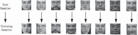
When the face recognition classifier is generated, the first five face images of each person are selected as training samples, and the last five face images are the test samples. The recognition results of some face test samples are shown in Fig. 4.6.

The experiment also compared the other algorithms in terms of the recognition rate. The comparison results are shown in Fig. 4.7. It can be seen that, as the number of training samples increases, the recognition rate of the three algorithms improves. PCA + LDA performs a PCA dimensionality reduction on the original image and then uses the LDA algorithm to identify the face image. This algorithm’s recognition rate is higher than that of the simple LDA algorithm. The performance of this algorithm is equivalent to that of PCA + LDA algorithm. When the number of training samples exceeds a certain threshold, our algorithm achieves a better recognition rate.

Tab. 4.6: DF form background of partial facial feature formation.

Fig. 4.6: Partial sample recognition result.

4.6.2Data classification experiments on UCI datasets

4.6.2.1Data classification experiments on UCI datasets

The second experiment used some datasets from the UCI-Machine-Learning database (see Tab. 4.7). The test sample set and the original dataset were preprocessed, and the training sample set and the test sample set were mixed. Cross-validation was used to test the constructed DF concept tree and the number of cross-validation directories was set to 10.

Some of the UCI datasets were tested by the C4.5 and DFDT algorithms. Depending on the constructed DF concept tree, pruning may or may not be performed. The number of concept nodes in the generated concept tree (a concept can have multiple concept nodes), the number of tree nodes, the correct number and accuracy of training samples, and the correct number and accuracy of cross-validation were recorded as evaluation metrics. The experimental results of the two algorithms are given in Tabs. 4.8 and 4.9. Figures 4.8 and 4.9 compare the accuracy of the algorithms based on the two results tables.

Tab. 4.7: UCI standard dataset information.

Fig. 4.7: Comparison of the recognition rates of the three algorithms.

Tab. 4.8: Experimental results of the C4.5 algorithm on the UCI dataset.

Tab. 4.9: Experimental results of DFDT algorithm on UCI dataset.

Fig. 4.8: Comparison of the classification accuracy of the classification algorithm on the training set.

4.6.2.2Analysis of results

The concept learning algorithm based on DFDT adopts the dynamic fuzzy preprocessing technique, which fully considers the dynamic fuzziness in the real problem and offers learning ability in the dynamic fuzzy environment. From the cross-validation concept classification accuracy rate, we can see that the prediction performance of concept classification is further improved over that of the C4.5 algorithm. In addition, when selecting the best classification attribute, the algorithm takes full account of the contribution of decision attributes to the whole set of decision instances, which can be used to classify the instances of unknown concept classes more precisely. Moreover, the size of the generated dynamic fuzzy leaf node (dynamic fuzzy concept node) and the tree size are smaller those that generated by the C4.5 algorithm. Therefore, the generalization ability of the constructed classifier is better, and the generalization ability has been enhanced.

Fig. 4.9: Cross-validation comparison of classification algorithms.

4.7Summary

This chapter has discussed the mechanism of a concept learning model based on DFS. According to the theory of DFS data modelling, a DF concept representation model was proposed. The formal representation of DF concepts was described by establishing the mapping relation between a DFD instance set and dynamic fuzzy attribute set (constituting the DFGalois connection).

References

[1]Mitchell TM. Version space: A candidate elimination approach to rule learning. In Proceedings of the Fifth international joint conference on AI, 1977, 305–310.

[2]Mitchell TM. Generalization as search. Artificial Intelligence, 1982, 18(2): 203–226.

[3]Valiant LG. A theory of the learnable. Communication of ACM, 1984, 27(11): 1134–1142.

[4]Duda R, Hart P. Pattern classification and science analysis. NY, USA, John Wiley and Sons, 1973.

[5]Littlestone N. Learning quickly when irrelevant attributes abound: A new linear-threshold algorithm. Machine Learning, 1988, 2(4): 285–318.

[6]Burusco A, Gonzalez RF. The study of the L-fuzzy concept lattice. Mathware and Soft Computing, 1994, 1(3): 209–218.

[7]Chein M. Algorithme de recherche des sou-matrices premières d’une matrice. Bulletin mathèmatique de la Sociètè des Sciences Mathèmatiques de la Rèpublique Socialiste de Roumanie, 1969, 13(1): 21–25.

[8]Bordat J P. Calcul pratique du treillis de Galois d’une correspondance. Matheìmatiques Informatiques Et Sciences Humaines, 1986, 96(96): 31–47, 101.

[9]Ganter B. Two basic algorithms in concept analysis. Lecture Notes in Computer Science, 2010, 5986: 312–340.

[10]Nourine L, Raynaud O. A fast algorithm for building lattice. Workshop on Computational Graph Theory and Combinations, Victoria, Canada, 1999.

[11]Godin R. Incremental concept formation algorithm bases on Galois (concept) lattices. Computational Intelligence, 1995, 11(2): 246–267.

[12]Carpineto C, Galois RG. An order-theoretic approach to conceptual clustering. In Proceedings of ICML-93, 1993, 33–40.

[13]Ho TB. Incremental conceptual clustering in the framework of Galois lattice. In Lu H, Motoda H, Liu H, eds. KDD: Techniques and Applications. Singapore: World Scientific, 1997, 49–64.

[14]Oosthuizen GD. Rough Sets and Concept Lattices. International Workshop on Rough Sets and Knowledge Discovery: Rough Sets, Fuzzy Sets and Knowledge Discovery. London: Springer-Verlag, 1993, 24–31.

[15]Agrawal R, Imielinski T, Swami AN. Mining Association Rules between Sets of Items in Large Databases. In Proceedings of the 1993 ACM SIGMOD International Conference on Management of Data, Washington, 1993, 207–216.

[16]Ho TB. An Approach to Concept Formation Based on Formal Concept Analysis. Ieice Transactions on Information & Systems, 1995, 78(5): 553–559.

[17]Qiang Y, Liu ZT, Lin W, et al. Research on fuzzy concept lattice in knowledge discovery and a construction algorithm. Acta Electronica Sinica, 2005, 33(2): 350–353.

[18]Shi ZZ. Knowledge discovery. Beijing, China, Tsinghua University Press, 2002.

[19]Huan L, Farhad H, Manoranjan D. Discretization: An enabling technique. Data Ming and Knowledge Discovery, 2002, 6(4): 393–423.

[20]Mao GJ, Duan LJ, Wang S, et al. Data mining principles and algorithms. Beijing, China, Tsinghua University Press, 2005.

[21]Witten IH, Frank E. Data mining practical machine learning tools and techniques with Java implementations. Beijing, China, China Machine Press, 2003.

[22]Liu XG. Research on the concept learning based on DFS. Master’s Thesis, Soochow University, Suzhou, China, 2011.

..................Content has been hidden....................

You can't read the all page of ebook, please click here login for view all page.

Table of Contents for 4.5.3 DF concept rule extraction and matching algorithm

Create new playlist

Sign In

Sign Up