Based on the existing examples in the real world, we conduct cooperative multiagent learning in two steps, common learning and comprehensive learning. The definition of common learning is that we set each agent to be an independent entity in the multi-agent system. Each agent completes its own task according to a particular single learning algorithm. An agent has properties such as independence and integrity. Independence means that each agent is an independent entity that is unaffected by other agents. Integrity means that each agent has a complete capacity for learning without any help from other agents. Comprehensive learning means that there is a comprehensive agent that manages every agent and obtains the optimal learning result in the shortest time. The comprehensive agent has properties such as comprehensiveness and sharing. Comprehensiveness means that the comprehensive agent can manage every agent in the learning system and assign different tasks to each agent. At the end of the mission, the comprehensive agent will choose the optimal learning sequence based on the reward value. Sharing means that each agent in the learning system has no need to complete all the learning tasks. This method will reduce the complexity of the agent.

At first, we define the common cooperative multi-agent learning model as

$<\left(agentt1,agent2,\dots ,agentn\right),\left(\left(\overleftarrow{S_0},\overrightarrow{S_0}\right)\left(\overleftarrow{S_g},\overrightarrow{S_g}\right)\right)>.\left(7.18\right)$

Here, we have a total of n agents, each with the same initial state and the same target state. In the multi-agent model, we concurrently conduct single-agent learning and orchestrate the multiple agents to form a system. Over a period of time, the state of the agents changes several times, from the initial state $\left({\overleftarrow{S}}_o,{\overrightarrow{S}}_o\right)$ to the present state $\left({\overleftarrow{S}}_g,{\overrightarrow{S}}_g\right)$ under the above learning method.

Secondly, the common cooperative multi-agent learning algorithm is as follows. In Algorithm 7.8, we assume that the agent has to conduct mi tests when state $({\overleftarrow{S}}_i,\overrightarrow{S_i})(0\le i\le g-1)$ is converted into state $({\overleftarrow{S}}_{i+1},\overrightarrow{S_{i+1}}).$ Then, the agent can decide which action best assist the change in state.

In Algorithm 7.8, we first finish the parallel learning mission for every agent and then group multiple agents to form the system. In this way, the time complexity of the grouping is lower than for parallel learning. Therefore, the time complexity of this method is T1 = t1 + t2 + ... + tn + telse, where telse is the extra time cost of operations such as grouping.

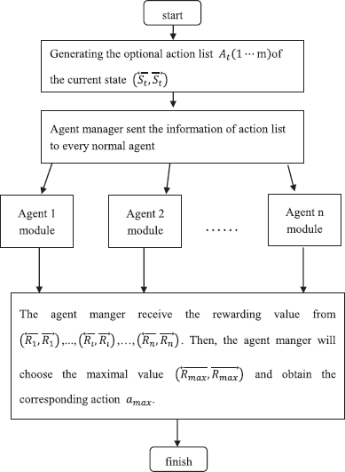
The above learning model does not take full advantage of the collaborative capacity of multiple agents to improve the learning speed. Now, we build a novel multi-agent collaborative learning model. In this new model, we assume there are n agents who learn together and execute some missions in parallel. To coordinate the learning tasks of n agents, the system has a special comprehensive agent, or agent manager. In Fig. 7.5, the double-sided arrow represents the communicating mechanism between agent i and the agent manager.

Agents 1 − n have the same structure. Each agent consists of three parts, a learner (L), motion converter (C), and state perceptron, and is connected with the agent manager. Normal agents can communicate with the agent manager, but there is no direct connection between them.

As well as these three basic modules, each agent has a status buffer that saves some intermediate results.

All agents, including the agent manager, have an identifier defined by the numbers 1 − n. Moreover, the strategy database and state of all the agents are the same.

The state perceptron of the agent manager estimates the action taken by each normal agent based on the current state information. Then, the agent manager combines these actions and forms an action list that is sent to every agent.

We set the initial reward value of agent $i(1\le i\le n)\text{to be}(\overleftarrow{r_1},\overrightarrow{r_1})=(\overleftarrow{0},\overrightarrow{0})$ and the other executable action ai to be null. When agent i receives the agent list from the agent manager, it executes action j in sequence. Action j meets the requirement that j mod n = i. During the execution, agent i saves the execution records. If $(\overleftarrow{r_1{}^{\prime }},\overrightarrow{r_1{}^{\prime }})>(\overleftarrow{r_1},\overrightarrow{r_1}),$ we set $(\overleftarrow{r_i},\overrightarrow{r_i})=(\overleftarrow{r_1{}^{\prime }},\overrightarrow{r_1{}^{\prime }}),a=a_i{}^{\prime }.$ When the agent has executed the action, it obtains the reward value $(\overleftarrow{r_i},\overrightarrow{r_i})$ and sends this value to the agent manager.

When the agent manager has received all reward value information from the normal agents, it chooses the maximal value and notifies every agent that this value has been obtained. Without loss of generality, we set the number of agents to be (1 ≤ u ≤ n). Agent u transmits the action corresponding to the maximal reward value to the agent manager. The agent manager notifies every agent using the broadcast mode. Each agent updates its own strategy database. By this method, each agent has learned the strategy corresponding to the maximal reward value. Fig. 7.6 shows the algorithm flowchart.

We can see from this figure that there is a processing module, called the module of agent i. The main work of this module is the corresponding management tasks when agent i receives the action list. The processing flowchart of this module is shown in Fig. 7.7.

In Algorithm 7.9, we can see that there are n agents and m executable actions. Each agent has to execute k actions. If the time required to execute action aj(1 ≤ j ≤ m) is tj and tmax = max (t1, t2, ..., tm), the execution time for all actions of agent i will be k*tmax. In addition, the agent manager will provide the action list and send it to every normal agent in broadcast mode. When the agent manager receives the reward values from the normal agents, it sends a notification that the time of the action corresponding to a strategy is telse. Each agent takes appropriate action when it receives the information of the maximal reward value. It is easy to see that tre ≤ tmax, so the time complexity of the algorithm is T2 1 ≤ k∗tmax telse tmax k tmax telse.

Example 7.5 We now analyse the comprehensive cooperative multi-agent learning algorithm. We take a classic machine learning problem, Sudoku, as an example.

In this example, we assume that there is an agent manager and four normal agents, numbered 1–4. The initial state is S0 and the target state is Sg in Fig. 7.8.

In this learning system, the computational method of the reward value is defined as follows: assume that a represents the different bits between the initial state and the target state and b represents the current depth. If the current state is not the target state, the reward value will be r = (10 − a − b)/10. If the different bits of the current state become the target state by proper angle rotation, the reward value will be $\overrightarrow{r};$ otherwise, it will be $\overleftarrow{r}.$ The action sequence of this problem consists of four directions, up, down, left, and right. Based on the above notation and preparation, we will solve the following problem.

(1)The agent manager obtains the action sequence (up, down, left, right) based on the initial state. This action sequence is sent to the four normal agents.

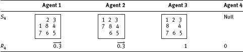
(2)Agents 1–4 conduct the four actions, respectively, and obtain four different states. The reward values are presented in Tab. 7.8.

(3)The agent manager receives the four reward values and chooses the maximal value R11. Then, the agent manager tells agent 1 to send its own action to the manager and to the other agents. Now, all the agents have the same action A1 = up and state S1 in Fig. 7.9. Thus, the system has a new state. The agent manager then obtains the new action set (down, left, right) based on the current state S1. Similar to the above method, the system will continue to search in Tabs. 7.9–7.11 and obtains A2 = left, State S2 in Fig. 7.9. The agent manager will obtain the new action sequence (down, right).

Tab. 7.8: Reward values of agents in state S1.

Tab. 7.9: Reward values of agents in state S2.

Tab. 7.10: Reward values of agents in state S3.

Finally, we obtain A4 = right and state S4. Because S4 = Sg, the system has reached the target state. The system terminates the learning process.

In the above example, there are two options in the process of converting state S0 into S1 without considering the dynamic fuzzy property. If the dynamic fuzzy property was considered, the search speed would be accelerated.

Tab. 7.11: Reward values of agents in state S3.

Example 7.6 This experiment will simulate a multi-agent system. During the learning process of the system, there are some optional actions numbered 1–4. These actions are selectable when the system is being converted to a new state. The execution time of each action is from 0 to 9 s. Now, we randomly generate 30 initial states. Each initial state can attain the target state. We employ a heuristic method and comprehensive multi-agent learning method. The results are presented in Tabs. 7.12–7.14 and Fig. 7.10.

It can be seen from Fig. 7.10 that the time complexity of the comprehensive multiagent learning method is far less than the heuristic method for larger numbers of experiments. Moreover, if the initial state repeatedly emerges or is an intermediate state, the time complexity of the learning will be zero, which means no work is required.

In the above algorithm, each agent is based on the real-time single-agent learning algorithm in a multi-agent system. However, Example 7.5 indicates that we can find a strategy to solve the problem using the single-agent learning algorithm, although this strategy is not optimal. Therefore, we need to employ the optimal strategy to construct the multi-agent system. Here, we employ Q-learning based on DFL to construct the cooperative multi-agent learning system.

Tab. 7.12: Execution time of action in state 1–10.

Tab. 7.13: Execution time of action in state 11–20.

Tab. 7.14: Execution time of action in state 21–30.

The Q-learning method has to consider that future actions will affect the current Q-value. Therefore, we employ the topological structure of the previous comprehensive multi-agent learning system. However, the internal structure of the agents is more complex. Each agent not only has the necessary intention database and the capacity database of the mental model, but also needs a stack and a queue. The stack is used to store the Q information of the agent to be processed. The queue is used to update the Q information for which each agent is responsible. The non-real-time cooperative multi-agent learning model is shown in Fig. 7.11.

The system has a comprehensive agent and several normal agents. These agents are arranged in a star-topology, which means that each agent can communicate with the other agents. Each agent has a database associated with its own mental state, for example, the belief database and the action database. To store some learning strategies, the system has a public strategy database. Employing the public strategy database, the system can directly call the corresponding strategy when the system encounters a similar state, thus avoiding any additional learning process.

Besides handling the overall planning of the system, the comprehensive agent acts as an interactive interface. Interacting with other agents through the comprehensive agent, the system then decides whether to conduct a learning process or provide the corresponding learning strategy to another agent system that needs to learn. The normal agents mainly depend on the overall planning of the comprehensive agent and learn the new strategy. At the same time, the normal agents will insert the latest strategy in their own databases. This updating method will help the system to perform well in the next learning process.

In general, the comprehensive agent gives corresponding instructions when it has received a specific message. Therefore, besides the basic function module of the mental state of the agent, it needs a message interrupting module. The interrupting module has a relatively simple function. The main algorithm flowchart is shown in Fig. 7.12.

However, the normal agent makes the corresponding action when it receives the instruction from the comprehensive agent. Without receiving the message, the normal agent also needs to conduct some learning process. The internal structure of the normal agent is relatively simple, which is shown in Fig. 7.13.

The learning module mainly conducts the learning task in the stack, which stores the learning task. The algorithm is show in Algorithm. 4.4 and the algorithm flow chart is show in Fig. 7.14.

The message interrupting module mainly conducts the message received by the agent. During the processing of the learning task, other agents would like to send some task instructions and learning results to the current agent. The message interrupting module needs to make corresponding response when it receives some related message. The algorithm flow chart is shown in Fig. 7.15.

It can be seen from the above algorithm that Q-learning is a kind of recursive approach. During the computing of $Q((\overleftarrow{s},\overrightarrow{s}),a),$ we need to compute the Q-value of the followup action a. Therefore, if we need to compute the Q-value m times to obtain the final result and the time complexity of each computation is t, the total time complexity of the algorithm is T = t∗[m/n]. The data structure of the queue node in the agent manager is defined as follows:

Here, Q(state, *) is the ID of the queue node. The agent ID is needed to define, for example, agent 1, agent 2, or agent 3. Hence, the agent ID of the field is 1, 2, or 3. The data structure of the queue node in the normal agent is defined as follows:

Here, Q(state, *) is the ID of the queue node. The Q-value is used to store the updated Q-value. Action is used to store the action that obtains the Q-value. The counter is used to count whether all actions have been calculated.

“Is it latest?” identifies whether the Q-value has been fully updated. If the Q-value has been updated, this value should be T. Otherwise, the value should be F. The data structure of the stack node in the normal agent is defined as follows. Here, Q(state, *) is the ID of the stack node.

Example 7.7 The initial setting of this example is the same as in Example 7.2. We explain Algorithms 4.3–4.5 in detail by solving the problem. First, we assume that the multi-agent system has four agents, numbered 1–4.

(1)Agents 1–4 initialize their stacks. The agent manager sends Q(1, *)to one agent.

(2)Select one agent at random to receive Q(1, *). In general, we set agent 1 to receive this information and push the value onto the stack of agent 1.

(3)All agents pop the pending nodes off their stacks. Agent 1 conducts the calculations for Q(1, *) and places the result into the corresponding queue. Agent 1 then sends Q(2, *), Q(3, *), Q(4, *) and Q(5, *) to the agent manager. The agent manager will judge whether these Q-values should be sent to the specific agents. If these Q-values are not sent to the specific agents, the agent manager will resend the information. Without loss of generality, we assume that agent i needs to conduct Q(i + 1, *), 1 ≤ i 4. When the other agents have no node calculations to conduct, the stacks of agents 1–4 contain Q(2, *), Q(3, *), Q(4, *) and Q(5, *), respectively.

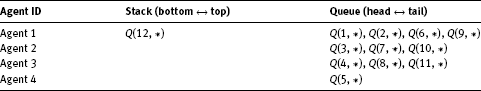
(4)When all agents pop the pending nodes off their stacks, agent i places Q(i + 1, *) into the corresponding queue. Agent i sends the corresponding Q-value to the agent manager. The agent manager coordinates all the Q-values and sends them to each agent. At this point, the queue and stack of each agent are as presented in Tabs. 7.15 and 7.16.

(5)All agents pop the pending nodes off their stacks and put them into the corresponding queues. The normal agents send the Q-values to the agent manager. The agent manager coordinates all the Q-values and sends them to each agent. The queue and stack of each agent are as given in Tabs. 7.17 and 7.18.

(6)All agents pop the pending nodes off their stacks and put them into the corresponding queues. The normal agents send the Q-values to the agent manager. The agent manager coordinates all the Q-values and sends them to each agent. The queue and stack of each agent are as given in Tabs. 7.19 and 7.20.

(7)All the agents pop the pending nodes off their stacks and put them into the corresponding queues. At this moment, the system will instantly compute the results and send them to agents 1–3.

(8)When we have Q(12, *), agents 1–3 calculate Q(9, *), Q(10, *), and Q(11, *), respectively. These results are then sent to the agents that need them.

(9)Each agent calculates Q(6, *), Q(7, *), and Q(8, ∗) based on the current received Q-value and sends the results to the agents that need them.

(10)Each agent calculates Q(2, *), Q(3, *), Q(4, *) and Q(5, *) based on the current received Q-value and sends the results to the agents that need them.

(11)Agent 1 calculates Q(1, *) and obtains the result.

(12)Finished.

Tab. 7.15: Queue and stack of each agent.

Tab. 7.16: Queue of the agent manager.

Tab. 7.17: Queue and stack of each agent.

Tab. 7.18: Queue of the agent manager.

Tab. 7.19: Queue and stack of each agent.

Tab. 7.20: Queue of the agent manager.

7.5Summary

Agent learning is a hot topic in many academic fields. The learning model of each agent follows a kind of dynamic fuzzy process. However, previous approaches do not solve dynamic fuzzy problems well. Therefore, this chapter has presented a kind of multi-agent learning model. The proposed model includes the mental model, immediate return single-agent learning algorithm, non-real-time cooperative multiagent learning model, cooperative multi-agent learning algorithm, and competitive multi-agent learning algorithm. The proposed model employs DFL theory to solve problems using agent learning.

The innovative points of this chapter include the following:

(1)We proposed a structure for the agent mental model based on DFL. The model structure is the foundation for researching agent learning.

(2)We proposed an immediate return single-agent learning algorithm and non-immediate return single-agent algorithm based on DFL. These methods are the foundation of further research on agent learning.

(3)Finally, we proposed a multi-agent learning model based on DFL. From the multiagent system, we developed cooperative and competitive multi-agent learning algorithms based on different relationships between the agents.

References

[1]Tan M. Multi-agent reinforcement learning: independent vs. cooperative agents. In Proceedings of Tenth International Conference on Machine Learning. San Francisco, Morgan Kaufmann, 1993, 487–494.

[2]Pan G. A framework for distributed reinforcement learning. In Proceedings of Adaption and learning in multi-agent system. Lecture Notes in Computer Sciences, NY, Springer, 1996, 97–112.

[3]Littman ML. Markov games as a framework for multi-agent reinforcement learning. In Proceedings of Eleventh International Conference on Machine Learning. New Brunswick, NJ, Morgan Kaufmann, 1994, 157–163.

[4]Roy N, Pineau J, Thrun S. Spoken dialogue management using probabilistic reasoning. In Proceedings of the 38th Annual Meeting of the Association for Computational Linguistics, 2000.

[5]Peter S, Manuela V. Team-partitioned, opaque-transition reinforcement learning. In Proceedings of the 3rd International Conference on Autonomous Agents. Seattle, ACM Press, 1999, 206–212.

[6]http://www.intel.com/research/mrl/pnl.

[7]Li FZ. Description of differential learning conception. Asian Journal of Information Technology, 2005, 4(3): 16–21.

[8]Tong HF. Design of auto-reasoning platform of multi-agent based on DFL. Master’s Thesis, Soochow University, Suzhou, China, 2005.

[9]Xie LP. Research on Multi-agent learning model based on DFL. Master’s Thesis, Soochow University, Suzhou, China, 2006.

[10]Xie LP, Li FZ. The mutil-agent learning model based on dynamic fuzzy logic. Journal of Communication and Computer, 2006, 3(3): 87–89.

[11]Bradshaw M. An introduction to software agents. Menlo Park, CA, MIT Press, 1997.

[12]Singh MP. Multi-agent systems: a theoretical framework for intention, know-how, and communication. Berlin, Germany: Springer-Verlag, 1994.

[13]Wooldridge M, Jennings NR. Intelligent agents: theory and practice. The Knowledge Engineering Review, 1995, 10(2): 115–152.

[14]Hu SL, Shi CY. Agent-BDI logic. Journal of Software, 2000, 11(10): 1353–1360.