Search in book...
Toggle Font Controls
Create new playlist

Name your new playlist

Playlist description (optional)
Sign In

Email address

Password

Forgot Password?

or

Continue with Facebook

Continue with Google
Sign Up

Full Name

Email address

Confirm Email Address

Password

or

Continue with Facebook

Continue with Google

Chapter 2

Hydraulic Fluid and Electrohydraulic Servo Valves

Different hydraulic fluids are used for different applications of electrohydraulic servo system. Components such as electrohydraulic servo valves, electrohydraulic servo mechanisms, sensors, etc. need to perform with different hydraulic fluids. It is first necessary to establish a mathematical model for the design and analysis of electrohydraulic servo valves. In this chapter, basic structure and working theory of electrohydraulic servo valves are introduced; the mathematical model of a two stage electrohydraulic servo valve with force feedback is analyzed, including the torque equilibrium equation of a torque motor, pressure-flow equation of a double nozzle flapper valve, torque equilibrium equation of an armature assembly and force equilibrium equation of a main spool, etc. The transfer function block diagram of electrohydraulic servo valves is established and simplified. This provides the basic model for the following model establishment, analysis and optimal design of electrohydraulic servo valves under vibration, impact and centrifugal conditions.

2.1. Hydraulic fluid in electrohydraulic servo systems

According to the required application, the most commonly used hydraulic fluids in electrohydraulic servo valve and electrohydraulic servo systems can be separated into jet fuel (fuel oil), hydraulic oil and phosphate ester hydraulic oil.

2.1.1. Jet fuel

I. Main grade of jet fuel

• RP-3 (3 # jet fuel, kerosene type)/GB 6537-1994.
• RP-5 (5 # jet fuel, common type or special test type)/GJB 560A-1997.
• RP-6 (6 # jet fuel, heavy kerosene type)/GJB 1603-1993.

II. Typical properties of hydraulic fluid

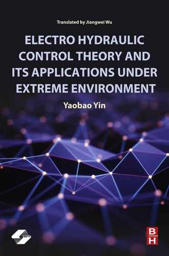
The main properties of RP-3 are represented in Table 2.1.

III. Characteristics and applications

Main characteristics:

• Low viscosity.
• Poor lubricity.
• Relatively poor thermal stability. Jet fuel is easily affected by the catalysis of copper alloy, which has adverse effects on the thermal stability of the material and increases the deterioration rate of the oil.
• High corrosivity. Jet fuel will corrode copper alloy, cadmium plating layers, etc. that are in contact with the fuel.
• Relatively high freezing point. Floc particles will form in the fuel at low temperatures.

Applications:

• Electrohydraulic servo valves in the engine of all types of subsonic and supersonic aircraft, helicopters, carrier-based aircraft, and auxiliary power, ground gas turbines use RP-3 fuel as hydraulic fluid.

Matters needing attention in application:

• Copper and copper alloys like bronze, brass, etc. cannot be used in the internal components of electrohydraulic fuel servo valves using jet fuel as hydraulic fluid that have contact with fuel oil.
• Coating technology like cadmium plating, nickel plating, etc. cannot be used in components in contact with fuel oil.
• Titanium alloy is not suitable for use in components of kinematic pairs in contact with fuel oil.
• Instatic and dynamic tests of electrohydraulic fuel servo valves, a flow meter or frequency test hydraulic cylinder that is suited to the fuel medium should be used in test equipment.

Table 2.1

Main properties of RP-3
Main properties		Parameters
Density (+20°C)/(kg/m³)		786.6
Kinematical viscosity (mm²/s)	20°C	1.55
Kinematical viscosity (mm²/s)	-20°C	3.58
Freezing point (°C)		-47
Flash point (°C)		45
Corrosivity (Copper corrosion, 2h/stage)		84% of grade 1a
Solid particle contamination (mg/l)		0.31

2.1.2. Hydraulic oil

I. Main grade of hydraulic oil

• 15 # aviation hydraulic oil (GJB 1177-1991).
• 12 # aviation hydraulic oil (Q/XJ 2007-1987).
• L-HM46 # anti-wear hydraulic oil (ISO 11158, GB 11118.1-94).

II. Typical properties of hydraulic fluid

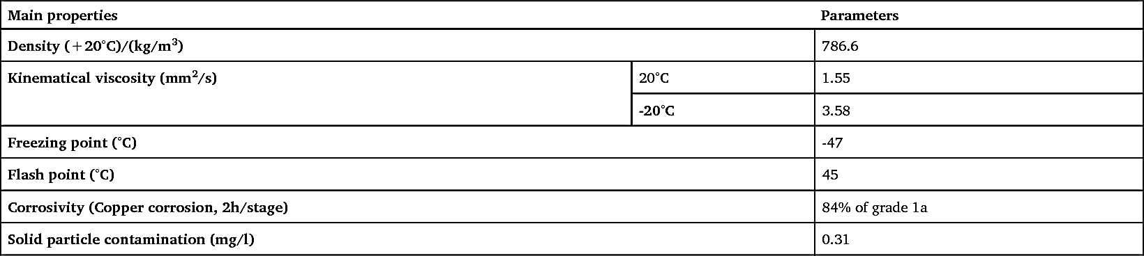
The main properties of 15 # aviation hydraulic oil are represented in Table 2.2.

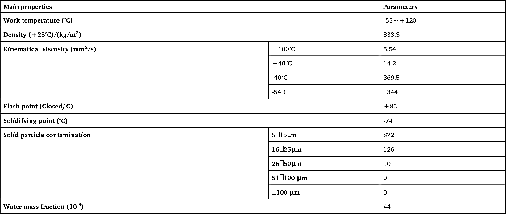
The main properties of YB-N68 # anti-wear hydraulic oil are represented in Table 2.3.

Table 2.2

Main properties of 15 # aviation hydraulic oil
Main properties		Parameters
Work temperature (°C)		-55∼+120
Density (+25°C)/(kg/m³)		833.3
Kinematical viscosity (mm²/s)	+100°C	5.54
	+40°C	14.2
	-40°C	369.5
	-54°C	1344
Flash point (Closed,°C)		+83
Solidifying point (°C)		-74
Solid particle contamination	5～15μm	872
	16～25μm	126
	26～50μm	10
	51～100 μm	0
	＞100 μm	0
Water mass fraction (10^-6)		44

Table 2.3

Main properties of YB-N68 # anti-wear hydraulic oil
Main properties		Parameters
Work temperature (°C)		-55～+120
Density (+25°C)/(kg/m³)		833.3
Kinematical viscosity (mm²/s)	+50°C	37～43
Kinematical viscosity (mm²/s)	+40°C	61.2～74.8
Flash point (Opened，°C)		＞+170
Solidifying point (°C)		＜-25

III. Characteristics and applications

Main characteristics:

• High viscosity. Viscosity decreases with increase in temperature; however, the rate of change in viscosity of aviation hydraulic oil is relatively small when the temperature is higher than 0˚C; that is, the viscosity-temperature characteristic is relatively good and has only a small effect on spray characteristics, jet characteristics and throttling characteristics of servo valves.
• Relatively high viscosity at low temperatures, making it easy to increase the resistance of moving parts like slide valve pairs in a servo valve.
• Good lubricity.
• Relatively good shearing stability.
• Relatively high density.

Applications:

• Hydraulic servo systems in ground equipment of the metallurgical and plastics industries and electrohydraulic servo valves in hydraulic servo systems of all types of construction machinery use anti-wear hydraulic oil and common mineral hydraulic oil.
• Electrohydraulic servo valves in hydraulic systems of all types of aircraft use 15 # aviation hydraulic oil as hydraulic fluid.

Matters needing attention in application:

• Ethylene-propylene rubber and butyl rubber cannot be used as glue stock for sealing elements inside electrohydraulic servo valves, due to compatibility problems.

2.1.3. Phosphate ester hydraulic oil

I. Main grade of phosphate ester hydraulic oil

• Skydrol LD-4 (SAE as 1241), 4611, 4613-1, 4614 phosphate ester hydraulic oil

II. Typical properties of hydraulic fluid

Phosphate ester hydraulic oil’s main properties are represented in Table 2.4.

III. Characteristics and applications

Main characteristics:

• Good flame resistance.
• Good oxidation safety.
• Good lubricity.
• High density.

Table 2.4

Main properties of phosphate ester hydraulic oil
Main properties		Parameters
Work temperature (°C)		-55～+120
Density (+25°C)/(kg/m³)		1.0009
Kinematical viscosity (mm²/s)	+38°C	11.42
	50°C (4613-1)	14.23
	50°C (4614)	22.14
	100°C	3.93
Flash point (°C)		171
Burning point (°C)		182

• Relatively high viscosity. The rate of change in viscosity with temperature is relatively large when the temperature is higher than 0˚C; that is, the viscosity-temperature characteristic is relatively poor, having a large effect on spray characteristics, jet characteristics and throttling characteristics of servo valves.

Applications:

• Electrohydraulic servo valves in hydraulic system of civil aircraft and ground gas turbines use phosphate ester hydraulic oil as hydraulic fluid.

Matters needing attention in application:

• 8350, 8360-1, 8370-1, 8380-1, H8901 ethylene-propylene-diene misch-polymere, fluoro rubber and silicon rubber should be used, and acrylonitrile-butadiene rubber and chloroprene rubber cannot be used as glue stock for sealing elements inside electrohydraulic servo valves, due to compatibility problems with phosphate ester hydraulic oil.

2.2. Principle and mathematic model of electrohydraulic servo valves

2.2.1. Principle of electrohydraulic servo valves

As the basis of properties analysis and optimal design of electrohydraulic servo valves, this section focuses on the force feedback electrohydraulic servo valve and its mathematic model. Fig. 2.1 is the schematic diagram of a two stage force feedback electrohydraulic servo valve. Force feedback electrohydraulic servo valves consist of two parts: a preamplifier stage consisting of a moving-iron torque motor and double nozzle flapper valve, and a slide valve power amplifier stage.

When the input control electric current

$Δ i = 0$

, the armature, supported by a spring, is evenly spaced between the upper and lower permanent magnets, and the flapper is evenly spaced between the two nozzles, the main spool is in the zero position and the electrohydraulic servo valve has no output. When the input control electric current has a value

$Δ i$

, the armature assembly deflects from the middle position, as does the flapper, the main spool deviates from the zero position, and the electrohydraulic servo valve opens and outputs corresponding pressure and flow. Changing the magnitude and direction of the control electric current changes the magnitude and direction of flow pressure correspondingly, as the magnitude of valve output and the deflection angle of the armature is in proportion to the control electric current. In Fig. 2.1, i ₁, i ₂ is the input control electric current; p ₁, p ₂ is the pressure of the main spool’s two ends; p _s is the pressure of oil supply; p _A, p _B is the pressure of loads input and output; p ₀ is the pressure of oil return.

Figure 2.1 Schematic diagram of a two stage force feedback electrohydraulic servo valve.

2.2.2. Fundamental equations of force feedback electrohydraulic servo valves

I. Classification and fundamental equations of permanent magnet torque motors

Classification of permanent magnet torque motors

Torque motor, an electro-mechanical conversion device, is the input stage of the electrohydraulic servo valve. It is classified into two types: moving-iron type and moving-coil type, according to its structure.

The permanent magnet moving-iron type torque motor is applied widely. As shown in Fig. 2.1, the moving-iron type torque motor consists of an armature that is installed on a torsion rod or spring tube and suspended in the air-gap of a magnetic field, a control coil, magnetizer (or yoke), and a permanent magnet (or magnet steel) etc. One of two pole terminals is magnetized to be N-pole; another one is magnetized to be S-pole. The magnetizer is set around the armature as a frame, to form a magnetic circuit. Magnetic flow via the armature is generated when an electric current passes through the control coil. Because this magnetic flow changes as the magnetic flux passes through four air-gaps, torque is generated and acts on the armature, making it turn around its axis or the rotation center of the spring tube; this force is in equilibrium with the reactive torque from the elastic support, therefore the armature rotates to a specific angular displacement. If the elastic support is a torsion rod, hydraulic oil can be used inside the torque motor, and this is called an immersed torque motor. If the elastic support is a spring tube, hydraulic oil cannot be used inside the torque motor, and this is called an air-gap torque motor.

Compared with the moving-coil type torque motor, the moving-iron type torque motor has a small inertia armature and large stiffness support spring tube, so has quick dynamic response. Under the same power, the natural frequency of the moving-iron type is about 15 times that of the moving-coil type. Under the same power and dimension, output force of the moving-iron type is about 7 times that of the moving-coil type. However, the moving-iron type is greatly affected by magnetic hysteresis and has significant nonlinearity. To restrict nonlinearity, the displacement of the armature should be quite small. Therefore, under the same conditions the linear range of moving-iron is about 1/3 of that of moving-coil.

Fundamental equations of torque motor

The input of a torque motor is the signal electric current into the control coil and the output is the rotation angle of the armature or the displacement of the flapper. If the two control coils in a torque motor have power supplied by a push-pull amplifier, the constant electric current produced by both control coils are equal in magnitude and opposite in direction, producing no torque acting on the armature and no deflection. As shown in Fig. 2.2, when a signal electric current is input, the electric current in one coil is reduced, making the respective currents in the two coils:

$i_{1} = i_{0} + i$

(2.1)

$i_{2} = i_{0} - i$

(2.2)

Figure 2.2 Permanent magnet torque motor driven by amplifier.

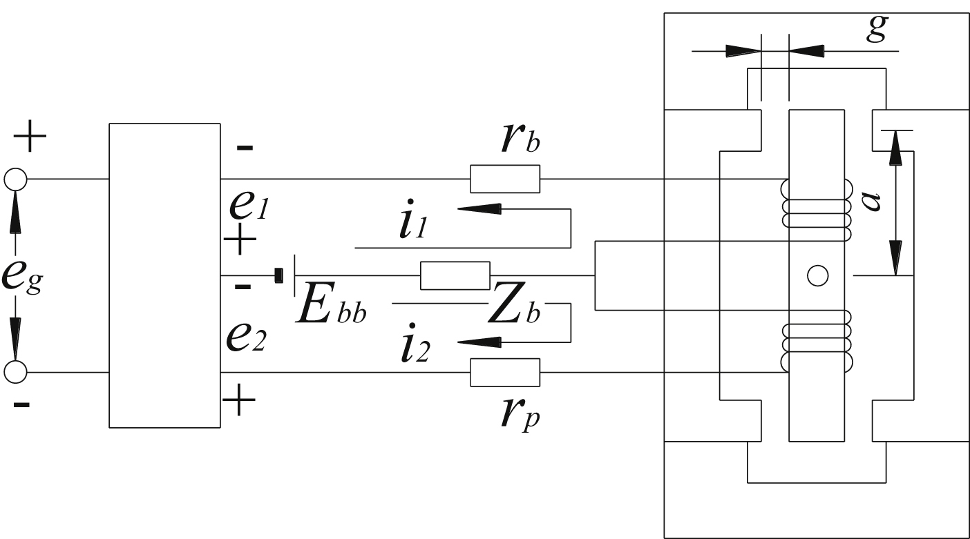
Subtracting the two equations:

$Δ i = 2 i = i_{1} - i_{2}$

(2.3)

where:

Δi is the differential current; that is the input of the torque motor;
I is the signal current;
i ₁ is the electric current in control coil 1;
i ₂ is the electric current in control coil 2; and
i ₀ is the constant electric current in each coil.

The two control coils of a torque motor can be connected in series or in parallel, and driven by a mono amplifier. The advantage of parallel connection is that the torque motor can still work when one coil is broken.

The working signal voltage of push-pull amplifier is:

$e_{1} = e_{2} = μ e_{g}$

(2.4)

where:

e ₁, e ₂ are the unilateral output voltages of the push-pull amplifier;
μ is the unilateral amplification factor of the push-pull amplifier; and
e _g is the signal voltage input of the push-pull amplifier.

The voltage equations for each control coil circuit are:

$E_{b} + e_{1} = i_{1} (Z_{b} + R_{c} + r_{p}) + i_{2} Z_{b} + N_{c} \frac{d Φ_{a}}{d t}$

(2.5)

$E_{b} - e_{2} = i_{2} (Z_{b} + R_{c} + r_{p}) + i_{1} Z_{b} - N_{c} \frac{d Φ_{a}}{d t}$

(2.6)

Subtracting Eq. (2.6) from Eq. (2.5), and substituting Eqs. (2.3) and (2.4), the fundamental equation of the torque motor is:

$2 μ e_{g} = (R_{c} + r_{p}) Δ i + 2 N_{c} \frac{d Φ_{a}}{d t}$

(2.7)

where:

R _c is the resistance of each control coil;
N _c is the number of windings of each control coil;
Φ_a is the total magnetic flow passing through the armature;
r _p is the internal resistance of the amplifier in each coil circuit;
E _bb is the voltage needed to produce a constant current; and
Z _b is the resistance of the common edge of the control coil.

Eq. (2.7) shows that the input voltage of the torque motor is consumed at two points. The first part of the equation indicates the voltage drop consumed in the control coil and by the internal resistance of the amplifier. The second part indicates the voltage drop due to the magnetic flow change in the armature caused by electromagnetic induction happening in the control coil as the current passes through. To find out the relationship between it and the angle displacement of the armature, it is necessary to find out the relationship between

$Φ_{a}$

and

$Δ i$

in Eq. (2.7) according to the magnetic circuit of the torque motor.

For convenience of analysis, it is assumed that the material’s reluctance in the magnetic circuit can be ignored, and air-gap reluctance on the cross is equal to each other. Four air-gap reluctances in Fig. 2.3, shown as ①, ②, ③ and ④, are predominating. According to the definition of reluctance, air-gap reluctances are:

$R_{1} = \frac{g - x}{μ_{0} A_{g}}$

(2.8)

$R_{2} = \frac{g + x}{μ_{0} A_{g}}$

(2.9)

where:

R ₁ is the reluctance of air-gaps ① and ②;
R ₂ is the reluctance of air-gaps ③ and ④;
g is the length of each air-gap when armature is in the middle position;
Figure 2.3 Magnet circuit schematic diagram of torque motor. (A) Magnet circuit schematic diagram (B) Equivalent magnet circuit schematic diagram.
x is the displacement of the top of the armature from the middle position;
A _g is the area of the air-gap plane; and
μ ₀ is the permeability of vacuum, the value is 4π×10⁻⁷H/m

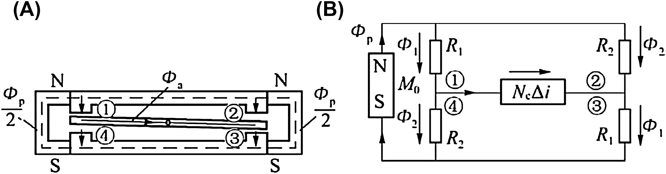
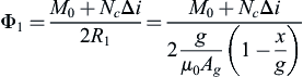
From the equivalent magnetic circuit in Fig. 2.3B, the magnetic flow of the air-gap on the cross is:

$Φ_{1} = \frac{M_{0} + N_{c} Δ i}{2 R_{1}} = \frac{M_{0} + N_{c} Δ i}{2 \frac{g}{μ_{0} A_{g}} (1 - \frac{x}{g})}$

(2.10)

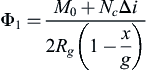
When the armature is in the middle position, the reluctance of the air-gap is:

$R_{g} = \frac{g}{μ_{0} A_{g}}$

(2.11)

From Eqs. (2.10) and (2.11), it is:

$Φ_{1} = \frac{M_{0} + N_{c} Δ i}{2 R_{g} (1 - \frac{x}{g})}$

(2.12)

Similarly:

$Φ_{2} = \frac{M_{0} + N_{c} Δ i}{2 R_{g} (1 + \frac{x}{g})}$

(2.13)

The magnetic flows passing through frame and armature are:

$Φ_{p} = Φ_{1} + Φ_{2}$

(2.14)

$Φ_{a} = Φ_{1} - Φ_{2}$

(2.15)

where:

Φ₁ is the magnetic flow passing through air-gaps ① and ③;
Φ₂ is the magnetic flow passing through air-gaps ② and ④;
M ₀ is the total magnetomotive force of all permanent magnets;
N _c Δ _i is the net magnetomotive force produced by the control current;
R _g is the reluctance of each air-gap when the armature is in the middle position;
Φ_p is the total magnetic flow passing through permanent magnets; and
Φ_a is the total magnetic flow passing through the armature.

It is more convenient to using air-gap magnetic flow when armature is in middle position represents M ₀. When the armature is in the middle position, Eqs. (2.12) and (2.13) can be simplified as:

$Φ_{10} = \frac{M_{0}}{2 R_{g}} = Φ_{20} = Φ_{g}$

(2.16)

where Φ_a is the magnetic flow of each air-gap when armature is in middle position.

So, the relationships between magnetic flows of air-gaps are:

$Φ_{1} = \frac{Φ_{g} + Φ_{c}}{1 - x / g}$

(2.17)

$Φ_{2} = \frac{Φ_{g} - Φ_{c}}{1 + x / g}$

(2.18)

where Φ_c is the magnetic flow produced by the control current.

It is decided by:

$Φ_{c} = \frac{N_{c} Δ i}{2 R_{g}}$

(2.19)

Substituting Eqs. (2.17) and (2.18) into Eq. (2.15), the relationship of magnetic flow inside the armature can be obtained:

$Φ_{a} = \frac{2 Φ_{g} (x / g) + 2 Φ_{c}}{1 - x^{2} / g^{2}}$

(2.20)

All torque motors are designed as x/g<1, so the equation above can be simplified as:

$Φ_{a} = 2 Φ_{g} \frac{x}{g} + \frac{N_{c}}{R_{g}} Δ i$

(2.21)

According to the geometrical relationship in Fig. 2.3A:

$t g θ = \frac{x}{a} \approx θ$

(2.22)

where:

θ is the angle displacement of the armature; and
α is the radius of armature from its axis to the center of the magnetizer working plane.

Because the deflection angle of the armature is small, the approximation relation in Eq. (2.22) is established normally. Combining Eqs. (2.21), (2.22) and (2.7) and rearranging, the voltage equation can be obtained as follows:

$2 μ e_{g} = (R_{c} + r_{p}) Δ i + 4 N_{c} Φ_{g} \frac{a}{g} \frac{d θ}{d t} + 2 \frac{N_{c}^{2}}{R_{g}} \frac{d Δ i}{d t}$

(2.23)

Applying Laplace transform to Eq. (2.23), there are:

$2 μ E_{g} = (R_{c} + r_{p}) Δ I + 2 K_{b} s θ + 2 L_{c} s Δ I$

(2.24)

$K_{b} = 2 (a / g) N_{c} Φ_{g}$

(2.25)

$L_{C} = N_{C}^{2} / R_{g}$

(2.26)

where:

K _b is the back electromotive force constant of each control coil; and
L _c is the coefficient of self-inductance of each control coil.

The above equation is the final form of the fundamental voltage equation of a torque motor. The equation of torque which is produced by the interaction between the magnetic flow of the permanent magnet and the air-gap controlling magnetic flow, and which acts on the armature, is derived in the following Maxwell equation:

$F = \frac{10^{7}}{8 π} \frac{Φ^{2}}{A_{g}}$

(2.27)

where:

F is the attractive force between two parallel magnetic planes separated by an air-gap;
Φ is the magnetic flow in the air-gap; and
A _g is the pole area perpendicular to the magnetic flow.

Because the directions of the torque produced in the two air-gaps in the end of the armature are opposite, the torque is proportional to the difference of two squares of magnetic flow, so the total net torque acting on the armature is:

$T_{d} = 2 a (Φ_{1}^{2} - Φ_{2}^{2}) \frac{10^{7}}{8 π A_{g}}$

(2.28)

The parameter, 2, in the above equation means that the two air-gaps on the other end produce the same torque too. Substituting Eqs. (2.17) and (2.18) into Eq. (2.28), x≈aθ、R _g=g/μ ₀ A _g and considering Φ_c=N _cΔi/2R _g, the torque equation can be obtained as follows:

$T_{d} = \frac{(1 + Φ_{c}^{2} / Φ_{g}^{2}) K_{m} θ + (1 + x^{2} / g^{2}) K_{t} Δ i}{{(1 - x^{2} / g^{2})}^{2}}$

(2.29)

$K_{t} = 2 (a / g) N_{c} Φ_{g}$

(2.30)

$K_{m} = 4 {(a / g)}^{2} Φ_{g}^{2} R_{g}$

(2.31)

where:

T _d is the total torque acting on the torque motor armature produced by the input current;
K _t is the torque constant of the torque motor; and
K _m is the magnetic spring coefficient of the torque motor.

Normally in torque motor design, (x/g)²<<1 and (Φ_c/Φ_g)<<1 is satisfied to improve its linearity, stability and prevent armature adsorbed by permanent magnet, so Equation (2.29) can be written as:

$T_{d} = K_{m} θ + K_{t} Δ i$

(2.32)

Applying Newton’s second law to the armature, the torque equilibrium equation of the armature can be obtained:

$T_{d} = J_{a} \frac{d^{2} θ}{d t^{2}} + B_{a} \frac{d θ}{d t} + K_{a} θ + T_{L}$

(2.33)

where:

J _a is the rotary inertia of the armature and its loads;
B _a is the viscous damping coefficient of the mechanical support and loads of the armature;
K _a is the torsion spring stiffness of the armature axis (or spring tube); and
T _L is the arbitrary torque load acting on the armature.

Combining Eqs. (2.32) and (2.33) and applying Laplace transform, the fundamental equation of the torque motor can be derived as:

$K_{m} θ + K_{t} Δ i = J_{a} \frac{d^{2} θ}{d t^{2}} + B_{a} \frac{d θ}{d t} + K_{a} θ + T_{L}$

$K_{t} Δ I = J_{a} s^{2} θ + B_{a} s θ + (K_{a} - K_{m}) θ + T_{L}$

(2.34)

From Eq. (2.33), it is necessary to keep the magnetic elastic coefficient smaller than the mechanical elastic constant in order to make the torque motor work stably.

II. Fundamental equations of double nozzle flapper valves

Flow pressure characteristic equation of double nozzle flapper valves

A double nozzle flapper valve is shown in Fig. 2.4. From the flow continuity equation of nozzle 1’s stream, there is:

$Q_{L} = Q_{1} - Q_{2}$

(2.35)

where:

Q ₁ is the flow passing through the fixed restrictor;
Q ₂ is the flow passing through nozzle 1; and
Q _L is the load flow.

From the flow pressure equation of the orifice, there are:

$Q_{1} = C_{d 0} A_{0} \sqrt{\frac{2}{ρ} (p_{s} - p_{1})} = \frac{1}{4} C_{d 0} π D_{0}^{2} \sqrt{\frac{2}{ρ} (p_{s} - p_{1})}$

(2.36)

$Q_{2} = C_{d f} π D_{N} (x_{f 0} - x_{f}) \sqrt{\frac{2}{ρ} p_{1}}$

(2.37)

where:

A ₀ is the throttling area of the fixed restrictor;
C _d0 is the flow coefficient of the fixed restrictor;
p _s is the pressure of the oil supply;
p ₁ is the cavity pressure of nozzle 1;
ρ is the density of the oil;
D _N is the diameter of the nozzle;
x _f0 is the original clearance between nozzle and flapper;
x _f is the moving distance of the flapper; and
C _df is the flow coefficient of the nozzle flapper orifice.

Similarly, when load is in a stable condition, a series of equations of another nozzle are:

$Q_{L} = Q_{4} - Q_{3}$

(2.38)

$Q_{3} = C_{d f} π D_{N} (x_{f 0} + x_{f}) \sqrt{\frac{2}{ρ} p_{2}}$

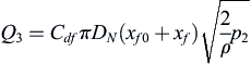(2.39)

$Q_{4} = C_{d 0} A_{0} \sqrt{\frac{2}{ρ} (p_{s} - p_{2})}$

(2.40)

where:

Q ₃ is the flow passing through the fixed restrictor;
Q ₄ is the flow passing through nozzle 2; and
p ₂ is the cavity pressure of nozzle 2.

Control valve normally work near its working point in hydraulic servo control system, therefore linearization of a double nozzle flapper valve is not required. According to the design criteria, the cavity control pressure of both nozzles is equal to 50% of oil supply pressure at the zero position. In this instance, the following equation of the fixed restrictor orifice and zero position nozzle flapper orifice must be satisfied:

$\frac{C_{d f} A_{f}}{C_{d 0} A_{0}} = \frac{C_{d f} π D_{N} x_{f 0}}{C_{d 0} A_{0}} = 1$

(2.41)

In order to determine valve parameters at the zero position, that is valve parameters at x _f=Q _L=p _L=0 and p ₁=p ₂=p _s/2, Eq. (2.35) is linearized as follows:

$Δ Q_{L} = \frac{\partial Q_{L}}{\partial x_{f}} Δ x_{f} + \frac{\partial Q_{L}}{\partial p_{1}} Δ p_{1}$

(2.42)

At the zero position, from the partial derivative of Eq. (2.35) and considering Eq. (2.41), there is:

${\frac{\partial Q_{L}}{\partial x_{f}} |}_{0} = C_{d f} π D_{N} \sqrt{\frac{p_{s}}{ρ}}$

(2.43)

${\frac{\partial Q_{L}}{\partial p_{1}} |}_{0} = - \frac{2 C_{d f} π D_{N} x_{f 0}}{\sqrt{ρ p_{s}}}$

(2.44)

From Eqs. (2.42)–(2.44), the following is obtained:

$Δ Q_{L} = C_{d f} π D_{N} \sqrt{\frac{p_{s}}{ρ}} Δ x_{f} - \frac{2 C_{d f} π D_{N} x_{f 0}}{\sqrt{ρ p_{s}}} Δ p_{1}$

(2.45)

Similarly, from Eq. (2.38), there is:

$Δ Q_{L} = C_{d f} π D_{N} \sqrt{\frac{p_{s}}{ρ}} Δ x_{f} + \frac{2 C_{d f} π D_{N} x_{f 0}}{\sqrt{ρ p_{s}}} Δ p_{2}$

(2.46)

Adding Eqs. (2.45) and (2.46), and combining Δp _L=Δp ₁-Δp _2, there is:

$Δ Q_{L} = C_{d f} π D_{N} \sqrt{\frac{p_{s}}{ρ}} Δ x_{f} - \frac{C_{d f} π D_{N} x_{f 0}}{\sqrt{ρ p_{s}}} Δ p_{L}$

(2.47)

This is the linearized equation of the pressure flow equation of a double nozzle flapper valve working at the zero position. The zero valve parameters can be obtained from the equation directly:

${K_{q 0} = \frac{\partial Q_{L}}{\partial x_{f}} |}_{Δ p_{L} = 0} = C_{d f} π D_{N} \sqrt{\frac{p_{s}}{ρ}}$

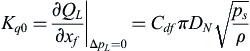(2.48)

${K_{p 0} = \frac{\partial p_{L}}{\partial x_{f}} |}_{Δ Q_{L} = 0} = \frac{p_{s}}{x_{f 0}}$

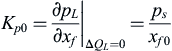(2.49)

${K_{c 0} = - \frac{\partial Q_{L}}{\partial p_{L}} |}_{Δ Q_{L} = 0} = \frac{C_{d f} π D_{N} x_{f 0}}{\sqrt{ρ p_{s}}}$

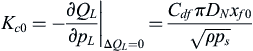(2.50)

Nozzle driving force of double nozzle flapper valves

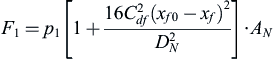
As shown in Fig. 2.4, the driving force of the jet-flow acting on the flapper can be obtained using the Bernoulli equation:

$F_{1} = (p_{1} + \frac{1}{2} ρ v_{1}^{2}) A_{N}$

(2.51)

where:

A _N is the cross sectional area of the nozzle orifice; and
v ₁ is the fluid velocity in the plane of nozzle export, it can be obtained by:

$v_{1} = \frac{Q_{2}}{A_{N}} = \frac{C_{d f} π D_{N} (x_{f 0} - x_{f}) \sqrt{(2 / ρ) p_{1}}}{π D_{N}^{2} / 4} = \frac{4 C_{d f} π (x_{f 0} - x_{f}) \sqrt{(2 / ρ) p_{1}}}{D_{N}}$

(2.52)

Combining the above two equations, there is:

$F_{1} = p_{1} [1 + \frac{16 C_{d f}^{2} {(x_{f 0} - x_{f})}^{2}}{D_{N}^{2}}] \cdot A_{N}$

(2.53)

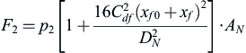
Similarly, the equation of F ₂ can be derived using a similar method:

$F_{2} = p_{2} [1 + \frac{16 C_{d f}^{2} {(x_{f 0} + x_{f})}^{2}}{D_{N}^{2}}] \cdot A_{N}$

(2.54)

Therefore, the net force acting on the flapper is the difference between these two forces:

$F_{1} - F_{2} = (p_{1} - p_{2}) A_{N} + 4 π C_{d f}^{2} [{(x_{f 0} - x_{f})}^{2} p_{1} - {(x_{f 0} + x_{f})}^{2} p_{2}]$

(2.55)

Using p _L=p ₁ − p ₂, and taking steady state value as p ₁≈p ₂≈p _s/2 approximately, there is:

$F_{1} - F_{2} = p_{L} A_{N} + 4 π C_{d f}^{2} x_{f 0}^{2} p_{L} + 4 π C_{d f}^{2} x_{f}^{2} p_{L} - 8 π C_{d f}^{2} x_{f 0} p_{s} x_{f}$

(2.56)

Normally, the design of flapper valves requires (x _f0/D _N)<1/16, that is, the area of the nozzle is far larger than the area of orifice formed by nozzle and flapper. That means the second part of equation can be ignored in favour of the first part. Here, because of x _f<x _f0, the third part of the equation is smaller than the second part, and can be ignored too. So, Eq. (2.56) can be written approximately as:

$F_{1} - F_{2} = p_{L} A_{N} - (8 π C_{d f}^{2} x_{f 0} p_{s}) x_{f}$

(2.57)

When the displacement of flapper x _f is small enough, angle θ is small too, so:

$t g θ = \frac{x_{f}}{r} \approx θ$

(2.58)

where r is the distance from axis of nozzle orifice to rotation center of armature.

From Eqs. (2.57) and (2.58), the load torque produced by double nozzle fluid forces in the electrohydraulic servo valve can be obtained as follows:

$T_{L e} = (F_{1} - F_{2}) r = p_{L} A_{N} r - r^{2} 8 π C_{d f}^{2} x_{f 0} p_{s} θ$

(2.59)

Equilibrium equation of flow

As shown in Fig. 2.1, the main spool can be considered as the load of the nozzle flapper valve in an electrohydraulic servo valve. Here, considering the compressibility of oil in the nozzle cavity, the equilibrium equation of flow and its Laplace transformation are, respectively:

$Q_{L} = A_{v} \frac{d X_{V}}{d t} + \frac{V_{o p}}{2 β_{e}} \frac{d P_{L}}{d t}$

$Q_{L} = A_{v} s X_{V} + \frac{V_{o p}}{2 β_{e}} s P_{L}$

(2.60)

where:

A _v is the end area of the spool;
V _op is the volume of one nozzle cavity when the spool is in the middle position;
X _V is the displacement of the main spool; and
β _e is the modules of elasticity of oil.

From Eqs. (2.47)–(2.50) and (2.58), the linear equation of flow transporting from nozzle flapper to main spool is:

$Q_{L} = K_{q 0} X_{f} - K_{c 0} P_{L} = K_{q 0} r θ - K_{c 0} P_{L}$

(2.61)

III. Torque equations of armature assembly

Fig. 2.5 is the working schematic diagram of an armature flapper feedback spring assembly.

It can be seen from the figure that the load torque from the force feedback bar to the armature is:

$T_{L K} = {(r + b)}^{2} K_{f} θ + K_{f} (r + b) x_{v}$

(2.62)

where:

Figure 2.5 Working schematic diagram of armature flapper feedback spring assembly.

K _f is the stiffness of the force feedback bar; and
b is the distance from the axis of the nozzle orifice to the axis of the main spool.

From Eqs. (2.59) and (2.60), the total load torque of the torque motor is:

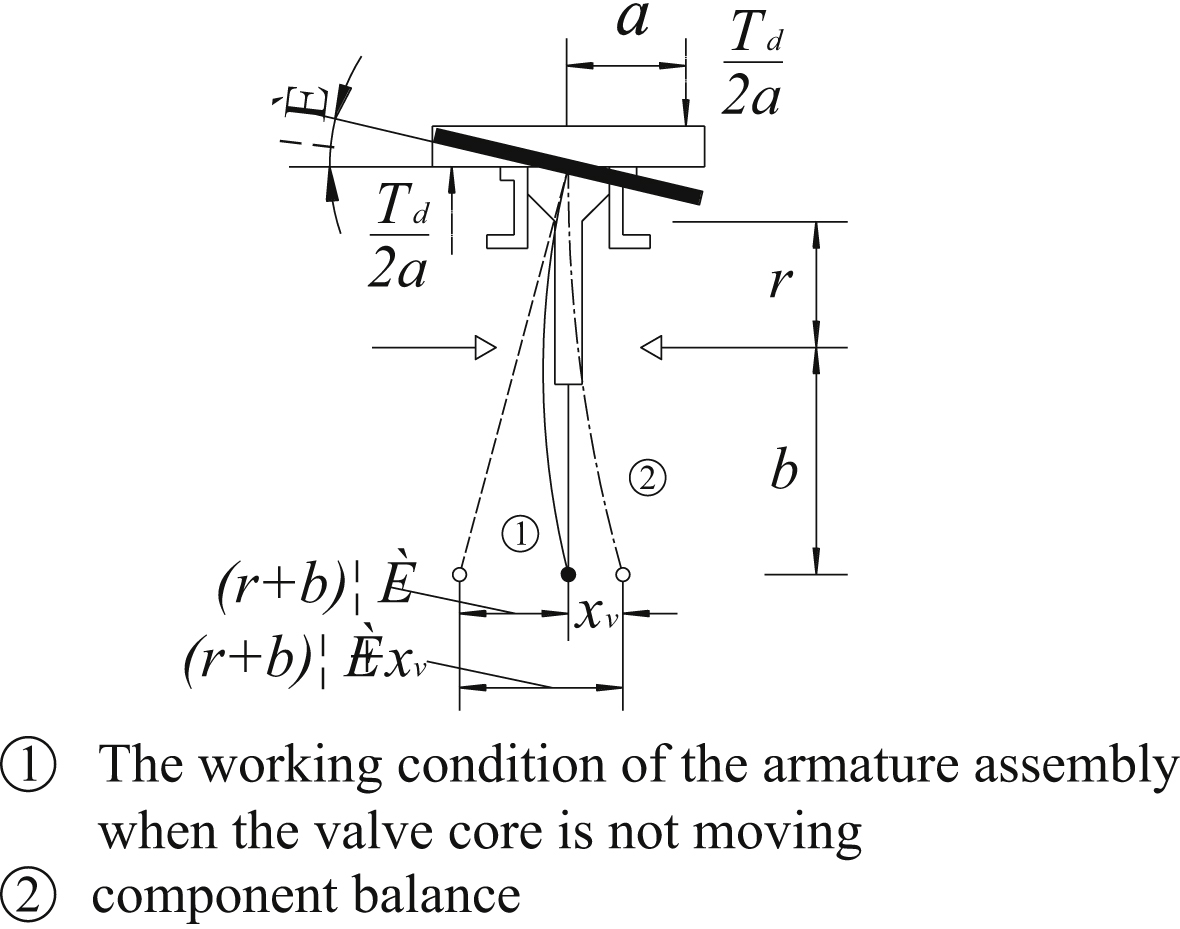
$T_{L} = r p_{L} A_{N} + {(r + b)}^{2} K_{f} θ + K_{f} (r + b) x_{v} - r^{2} 8 π C_{d f}^{2} x_{f 0} p_{s} θ$

(2.63)

Transforming Eq. (2.63) using Laplace transform, and substituting into Eq. (2.34), the torque equations of armature assembly are:

$K_{t} Δ I = J_{a} s^{2} θ + B_{a} s θ + [K_{a n} + K_{f} {(r + b)}^{2}] θ + K_{f} (r + b) X_{V} + r P_{L} A_{N}$

(2.64)

where K _an is the net stiffness coefficient of the armature flapper.

$K_{a n} = K_{a} + K_{m} - 8 π C_{d f}^{2} p_{s} x_{f 0} r^{2}$

(2.65)

Eq. (2.64) can be rewritten as:

$θ = \frac{\frac{1}{K_{a n} + K_{f} {(r + b)}^{2}} [K_{t} Δ I - K_{f} (r + b) X_{V} - r A_{N} P_{L p}]}{\frac{s^{2}}{ω_{m f}^{2}} + \frac{2 ζ_{m f}}{ω_{m f}} s + 1}$

(2.66)

$ω_{m f} = \sqrt{\frac{K_{a n} + K_{f} {(r + b)}^{2}}{J_{a}}}$

(2.67)

$ζ_{m f} = \frac{B_{a}}{2 \sqrt{J_{a} [K_{a n} + K_{f} {(r + b)}^{2}}}$

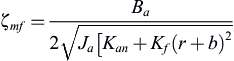(2.68)

where:

ω _mf is the natural frequency of the torque motor; and
ζ _mf is the damping ratio of the torque motor.

IV. Force equilibrium equation of main spool

Applying Newton’s second law to the main spool, the force equilibrium equation of the main spool is obtained as:

$A_{v} P_{L} = m_{v} s^{2} X_{V} + B_{v} s X_{V} + (K_{f} + {K^{'}}_{f}) X_{V}$

(2.69)

where:

m _v is the mass of the output stage spool;
B _v is the kinematical viscosity damping coefficient of the spool; and
K _f′ = 0.43ω(p _s-p _L0) is the dynamic stiffness of fluid acting on the spool.

2.2.3. Transfer functions of force feedback electrohydraulic servo valves

I. Transfer functions of electrohydraulic servo valves

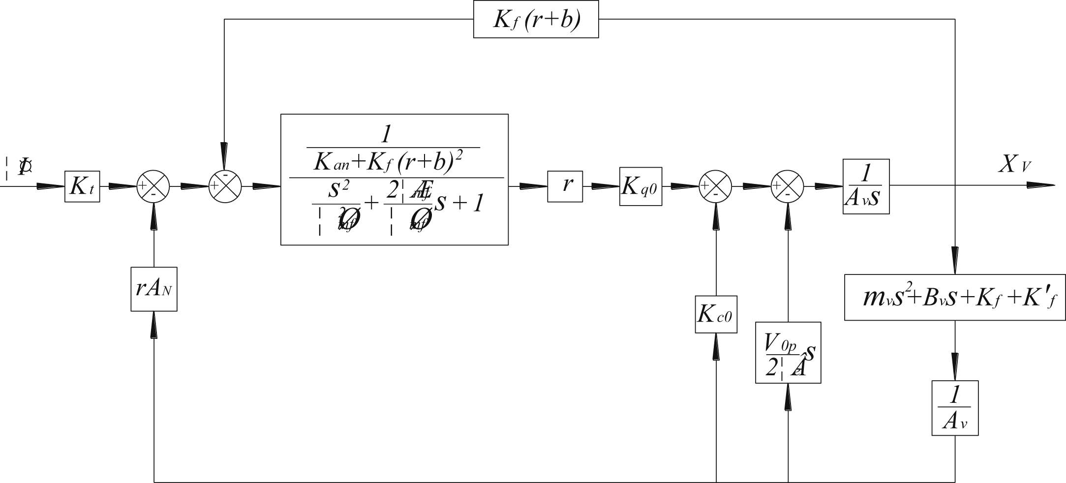
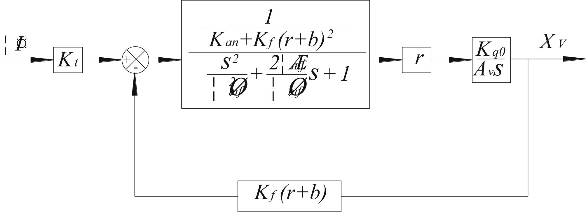
From Eqs. (2.60)–(2.62) and (2.69), the block diagram of an electrohydraulic servo valve with current input and displacement of main spool output is shown in Fig. 2.6. The hydraulic natural frequency of the two-step element, which consists of spool mass, fluid compressibility and pressure-flow coefficient of nozzle flapper valve, is quite high, so has basically no effect on dynamic quality. The maximum value of the open-loop gain function of the pressure feedback loop formed of spool movement is much smaller than the value of the open-loop gain of the force feedback loop. Therefore, it can be ignored. So, Fig. 2.6 can be simplified as shown in Fig. 2.7.

From Fig. 2.7, the open-loop transfer function of a force feedback two stage electrohydraulic servo valve is:

$G (s) H (s) = \frac{K_{v f}}{s (\frac{1}{{ω_{m f}}^{2}} s^{2} + \frac{2 ξ_{m f}}{ω_{m f}} s + 1)}$

(2.70)

where K _vf is the amplification coefficient of velocity; it is:

Figure 2.6 Block diagram of force feedback two stage electrohydraulic servo valve with current input.

Figure 2.7 Simplified block diagram of force feedback two stage electrohydraulic servo valve.

$K_{v f} = \frac{r (r + b) K_{f} K_{q 0}}{A_{v} [K_{a n} + K_{f} {(r + b)}^{2}]}$

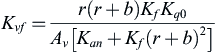(2.71)

Its close-loop transfer function is the transfer function of a force feedback two stage valve with current input and displacement of main spool output. It is:

$G_{B} (s) = \frac{X_{V}}{Δ I} = \frac{\frac{K_{t}}{K_{f} (r + b)}}{\frac{1}{K_{v f} ω_{m f}^{2}} s^{3} + \frac{2 ξ_{m f}}{K_{v f} ω_{m f}} s^{2} + \frac{1}{K_{v f}} s + 1}$

(2.72)

II. Analysis of stability

Its characteristic equation can be obtained from the open-loop transfer function (2.70) of a force feedback two stage electrohydraulic servo valve:

$\frac{1}{ω_{m f}^{2}} s^{3} + \frac{2 ξ_{m f}}{ω_{m f}} s^{2} + s + K_{v f} = 0$

(2.73)

According to the Routh-Hurwitz criterion, its stability criteria is:

$\frac{K_{v f}}{ω_{m f}} < 2 ξ_{m f}$

(2.74)

..................Content has been hidden....................

You can't read the all page of ebook, please click here login for view all page.

Table of Contents for Chapter 2. Hydraulic Fluid and Electrohydraulic Servo Valves

Create new playlist

Sign In

Sign Up

2.1. Hydraulic fluid in electrohydraulic servo systems

2.1.1. Jet fuel

I. Main grade of jet fuel

II. Typical properties of hydraulic fluid

III. Characteristics and applications

2.1.2. Hydraulic oil

I. Main grade of hydraulic oil

II. Typical properties of hydraulic fluid

III. Characteristics and applications

2.1.3. Phosphate ester hydraulic oil

I. Main grade of phosphate ester hydraulic oil

II. Typical properties of hydraulic fluid

III. Characteristics and applications

2.2. Principle and mathematic model of electrohydraulic servo valves

2.2.1. Principle of electrohydraulic servo valves

2.2.2. Fundamental equations of force feedback electrohydraulic servo valves

I. Classification and fundamental equations of permanent magnet torque motors

Classification of permanent magnet torque motors

Fundamental equations of torque motor

II. Fundamental equations of double nozzle flapper valves

Flow pressure characteristic equation of double nozzle flapper valves

Nozzle driving force of double nozzle flapper valves

Equilibrium equation of flow

III. Torque equations of armature assembly

IV. Force equilibrium equation of main spool

2.2.3. Transfer functions of force feedback electrohydraulic servo valves

I. Transfer functions of electrohydraulic servo valves

II. Analysis of stability

Table of Contents for
Chapter 2. Hydraulic Fluid and Electrohydraulic Servo Valves