The specific situation we will consider consists of a publisher or advertising network that displays ads—ours as well as those from competing advertisers. We cannot directly control how often our ads are shown. Instead, we can name the maximum price that each showing (or impression) is worth to us, after which the publisher will make a selection based on this offer. All we know is that a higher offered price tends to result in a greater number of ad impressions.

The system we want to control is the publisher. The control input is the price, and the control output is the number of impressions served. Knowing that a higher price means more impressions provides the tiny but necessary bit of process knowledge required to set up a feedback scheme.

I assume that we can set our price once every 24 hours and that we will learn the outcome (that is, the number of impressions truly delivered for this price) by the end of that period. Of course, there is nothing magical about the 24-hour period—any other fixed time (such as 6 hours or 48 hours) would work as well. What is relevant is that we will not learn about the results of the most recent run until the moment we have to choose a new input. This kind of dynamics is typical of computer systems but is quite unlike the behavior of items in the physical world: instead of a gradual response to a control input, we get a steplike response that is complete but delayed by one time step.

The setpoint for this control problem consists of the number of impressions we wish to generate every day. Let’s suppose that we already have a plan that spells this number out.

There is very little that we know offhand about the process that we want to control except for the directionality of the input/output relationship (higher prices lead to a greater number of impressions). In the first step, we measure the static process characteristic (Chapter 8).

For several values of the input (the price), we observe the resulting output (the number of impressions). Since the number of impressions will fluctuate from day to day because of the randomness of web traffic, we should repeat every measurement several times. The results might look like Figure 14-1.^[15] There is a minimum price that needs to be offered to receive any traffic; for higher prices, we see that the number of delivered impressions grows with the price but not linearly. The range of outcomes for each fixed price gives us an estimate for the amplitude of the day-to-day fluctuations. So far, so good.

Figure 14-1 looks simple, but it hides a great deal of practical difficulty. Recall that we must wait an entire day for each data point in the graph. The figure shows 10 trials for each price, and a total of 100 different prices. If we conduct this experiment sequentially, it will take three years to collect all the data—by which time most of it will be obsolete. It is clear that most of the time we will have to content ourselves with much less complete test coverage—perhaps just two or three data points to find the order of magnitude of the quantities involved. (The inability to run exhaustive experiments is a recurrent issue when working with control systems.)

Figure 14-1. The static process characteristic: if we are willing to pay a certain price per impression, how many impressions do we obtain?

We do not need to conduct an experiment to find the dynamic response of the system because we already know it: full response, but one day later. This is enough to set up a basic control loop.

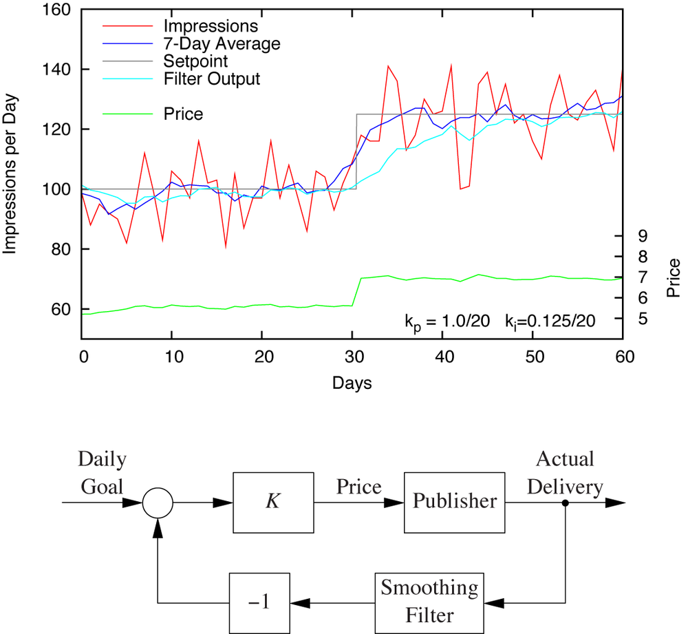
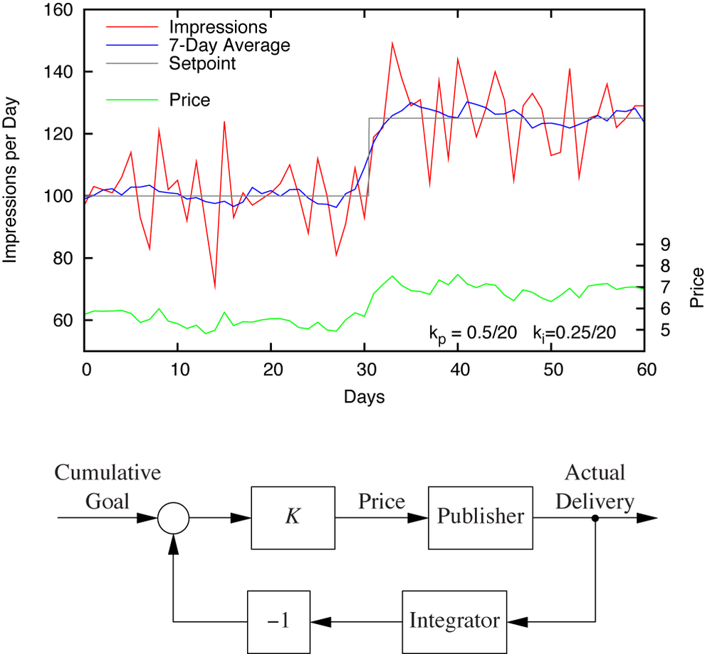
To establish control, we set up a basic control loop for our system using a standard PID controller K. The controller converts the difference between the daily impression goal (the setpoint) and the number of impressions actually delivered on the previous day into a new price, which is then passed to the publisher (see Figure 14-2).

In order to make things concrete, we must choose numerical values for the gain parameters in the PID controller. Unfortunately, none of the tuning methods discussed in Chapter 9 seem to be of much help. These methods all assume that there is a measurable delay τ and a time constant T in order to arrive at numerical values that can be used in a control loop implementation. In the present situation, however, the response is instantaneous. What should we do?

Figure 14-2. Loop architecture for the current case study.

The situation is actually much simpler than it may appear. Near the end of Chapter 9 we saw that all the tuning formulas could be written in the form

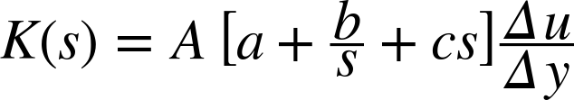
where Δu is the static change in control input needed to bring about a change Δy in the steady-state control output. The factor A is an adjustment to the static input/output relation that takes the system dynamics into account.

In the present situation, we are trying to control a system that has no (nontrivial) dynamics: it responds immediately. In other words, there is no need for the dynamic adjustment factor in the controller—we can basically ignore the A factor.

The static factor Δu/Δy can be obtained directly from the process characteristic: Figure 14-1 tells us that if we start with a price of $5, then a change by Δu = ±$1 will result in a change in output of roughly Δy = ± 20 impressions; therefore,

Finally, we will choose (somewhat arbitrarily)

as values for the term-specific coefficients (inside the central brackets). The actual controller gains consist of the combination of this coefficient with the static gain:

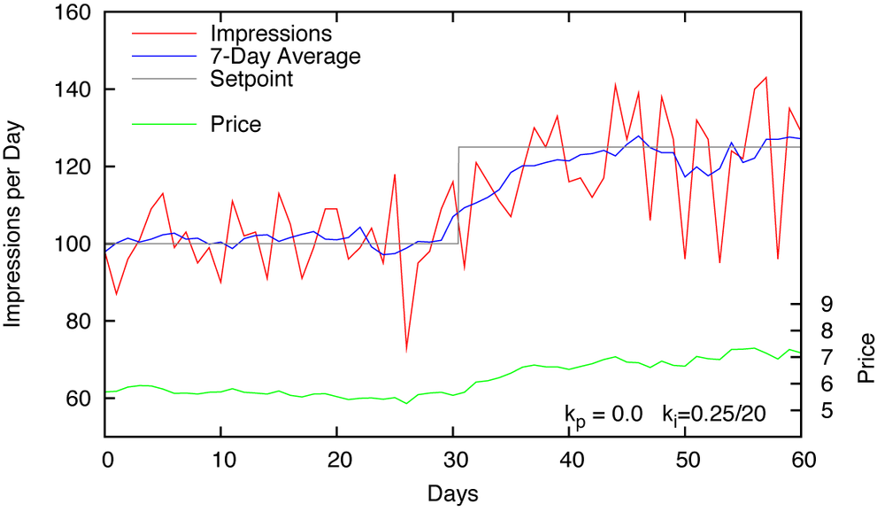
The behavior that is found when a controller with these specifications is placed into the loop is shown in Figure 14-3. As we can see, the performance is not great but is entirely acceptable.

Figure 14-3. Performance of the closed loop when using the “default” controller gains.

Looking at Figure 14-3, we can see that the system does track the set-point and responds to the setpoint change reasonably quickly (within four to five days). But the daily fluctuations in process output are large (as much as ±30 percent). What is worse, the process input also fluctuates. If there is a fixed fee or administrative cost associated with each price change that we submit to the publisher, such noisy behavior is clearly undesirable.

In an attempt to make the system less noisy, we might try to reduce the proportional term and rely more on the slower-acting integral term. In fact, we can dispense with the proportional term entirely! As long as the setpoint does not change for several days at a time, the changes in the tracking error from one day to the next are due entirely to random fluctuations in the web traffic. In the present situation, fluctuations on consecutive days are statistically independent; hence there is no way to predict tomorrow’s value from today’s. So the proportional term, which acts on the current value of the tracking error, is useless: there is no way that the momentary value of the tracking error can be used to reduce the tracking error in the future.

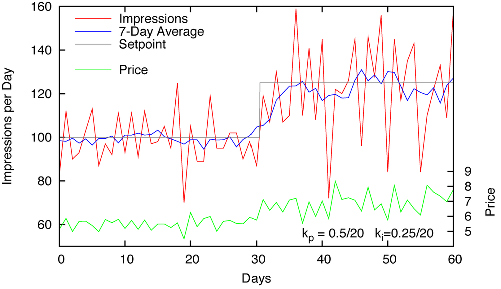
Figure 14-4 and Figure 14-5 show the system under strictly integral control. In Figure 14-4, the integral gain is the same as in Figure 14-3 (k_i = 0.25/20) but the proportional gain is now zero (k_p = 0). Compared to the previous situation, the amplitude of the noise has been reduced and the price (the control input) is much steadier; however, the system is also more sluggish.

Figure 14-4. Performance of the closed loop under strictly integral control. For k_i = 0.25/20, the behavior is sluggish: it takes more than 10 days to adjust fully to the setpoint change.

Whereas before it reacted to a setpoint change within a few days, now it takes well over 10 days to fully adjust to a new setpoint value. This is a problem—advertising campaigns typically only run for weeks or months, so a delay that exceeds a week is probably not acceptable.

We might try improving the system’s responsiveness by increasing the integral gain, but any increase in speed comes at the expense of increased instability: the system begins to oscillate wildly from one time step to the next (Figure 14-5). This is a common problem in control systems with discrete time steps and immediate-response dynamics. Because there is no partial response, the system easily falls into this particular type of rapid control oscillation if the corrective actions are too large. That tendency imposes relatively tight limits on the controller gains we can use in systems of this kind.

Figure 14-5. Performance of the closed loop under strictly integral control. Increasing the controller gain to k_i = 1.75/20 leads to control oscillations.

These observations already suggest the solution: we need to introduce a filter that will slow things down and “round off” the responses. This results in a loop architecture like the one shown in Figure 14-6 (bottom). A recursive filter

is introduced into the return path. The filter output lags behind but is also smooth, so it makes sense to use proportional control again in order to speed up the response. With k_p = 1.0/20 and k_i = 0.125/20, the observed behavior seems to strike a good balance (Figure 14-6, top). Notice in particular how little the price changes over time—except for the sudden (and properly sized) jump in response to the setpoint change.

Figure 14-6. The effect of including a smoothing filter into the loop. Now that the signal is smooth, it makes sense to include proportional control again.

The solution just presented seems satisfactory, but there are additional variations and enhancements that we don’t explore in detail in this case study. Some directions are summarized next.

Cumulative Goal

In the preceding solution, we used the daily impression target as setpoint. We can slice the problem differently by using the cumulative impression target as setpoint. From a business perspective, this is arguably a more meaningful design because the quantity that we ultimately want to control is usually the number of impressions served over the entire duration of a campaign—the daily target is merely derived from that.

In order to use the cumulative target, we must insert an additional integrator into the return path of the control loop (Figure 14-7, bottom). The process continues to report the number of impressions served per day and the integrator adds them up, reporting the cumulative impressions served, so that their value can be compared to the cumulative goal. Of course, the setpoint must now steadily increase in value. The resulting behavior is shown in Figure 14-7 (top). (For graphing purposes, the daily setpoint value is shown.) We should keep in mind, however, that this solution has few (if any) advantages over the one using a daily goal and a smoothing filter. The integrator just introduced merely replicates the behavior of the controller’s integral term in the previous solution.

Figure 14-7. Including an integrator on the return path while using the cumulative instead of the daily goal. In this scenario, the setpoint is not constant but instead is a ramp input.

The model for the publisher that was used in the simulations is given next. Its primary responsibility is to create a value for the “impressions delivered,” given a “price.” For the purpose of this simulation, I create the number of impressions as random numbers drawn from a Gaussian distribution. The mean of the distribution depends logarithmically on the price. (The latter choice is common in decision-theoretic modeling: the “value” of an item increases only logarithmically with the price, as when a car that is 10 times more expensive can only drive twice as fast.) Please keep in mind that this implementation is only a model that has been chosen to demonstrate the basic process. Other choices could (and possibly should) be made.

include math
include random
include feedback as fb

class AdPublisher( fb.Component ):

    def __init__( self, scale, min_price, relative_width=0.1 ):
        self.scale = scale
        self.min = min_price
        self.width = relative_width

    def work( self, u ):
        if u <= self.min:    # Price below min: no impressions
            return 0

        # "demand" is the number of impressions served per day
        # The demand is modeled (!) as Gaussian distribution
        # with a mean that depends logarithmically on the
        # price u.

        mean = self.scale*math.log( u/self.min )
        demand = int( random.gauss( mean, self.width*mean ) )

        return max( 0, demand ) # Impression demand is greater
                                # than zero.

We can use this definition of the AdPublisher to form a control loop, using a PID controller and one of the convenience functions from the simulation framework:

def closedloop( kp, ki, f=fb.Identity() ):
    def setpoint( t ):
        if t > 1000:
            return 125
        return 100

    k = 1.0/20.0

    p = AdPublisher( 100, 2 )
    c = fb.PidController( k*kp, k*ki )

    fb.closed_loop( setpoint, c, p, returnfilter=f )

We need to select the length of the time step before we can run the simulation. We perform one control action per day. If we measure time in days, then the length of each step is equal to 1.

Running the closed loop arrangement, including the smoothing filter, can then be accomplished using the following call:

fb.DT = 1

closedloop( 1.0, 0.125, fb.RecursiveFilter(0.125) )