We will consider different systems in this book that serve a variety of purposes. What these systems have in common is that all of them depend on configuration or tuning parameters that affect the system’s behavior. To obtain knowledge about that behavior, we track or observe various monitored metrics. In most cases, the system is expected to meet or exceed some predefined quality-of-service measure. The control problem therefore consists of adjusting the configuration parameters in such a way that the monitored metrics fall within the range prescribed by the quality-of-service requirements.

As far as the control problem is concerned, the configuration parameters are the variables that we can influence or manipulate directly. They are sometimes called the manipulated variables or simply the (control) inputs. The monitored metrics are the variables that we want to influence, and they are occasionally known as the process variables or the (control) outputs. The inputs and outputs taken together constitute the control signals.

The terms “input” and “output” for (respectively) the manipulated and the tracked quantities, are very handy, and we will use them often. However, it is important to keep in mind that this terminology refers only to the purpose of those quantities with respect to the control problem and so has nothing to do with functional “inputs” or “outputs” of the system. Whenever there is any risk of confusion, use the terms “configurable parameter” and “tracked metric” in place of “input” and “output.”

For the most part we will consider only those systems that have exactly one control input and control output, so that there is only a single configurable parameter that can be adjusted in order to influence the a single tracked metric. Although this may seem like an extreme limitation, it does cover a wide variety of systems. (Treating systems that have multiple inputs or outputs is possible in principle, but it poses serious practical problems.)

Here is a list of some systems and their input and output signals from enterprise programming and software engineering.

Other examples:

The feedback principle demands that the process output be constantly compared to the reference value (usually known as the setpoint). The deviation of the actual process output from the setpoint is the tracking error:

The job of the controller in Figure 2-1 is to calculate a corrective action based on the value of the tracking error. If the tracking error is positive (meaning that the process output is too low) then the controller must produce a new control input that will raise the output of the process, and vice versa.

Observe that the controller can do this without detailed knowledge about the system and its behavior. The controller mainly needs knowledge about the directionality of the process: does the input need to be increased or decreased in order to raise the output value? Both situations do occur: increasing the power supplied to a heating element will lead to an increase in temperature, but increasing the power supplied to a cooler will lead to a decrease!

Once the direction for the control action has been determined, the controller must also choose the magnitude of the correction. We will have more to say on this in the next section.

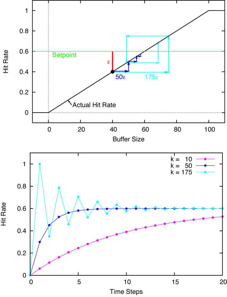
The introduction of a feedback loop can make an originally stable system unstable. The problem is usually due to persistent overcompensation, which results from corrective actions that are too large. Consider the cache (from the examples listed previously) and assume that the hit rate is initially below the desired value. To increase the hit rate, we need to make the cache larger. But how much larger? If we make the cache too large, then the hit rate will end up being above the desired value so that the cache size ends up being reduced in the next step; and so on. The system undergoes control oscillations, switching rapidly and violently between different configurations; see Figure 2-3.

Control oscillations are rarely desirable—just imagine the cruise control in your car behaving this way! But things can get worse: if each over- or undershoot leads to an even larger compensating action, then the amplitude of the oscillations grows with time. The system has thus become unstable and will break up (or blow up) before long. Such unstable behavior must be avoided in control loops at all cost.

The opposite problem is slow or sluggish behavior. If we are too timid and apply control actions that are too small, then the system will be slow to respond to disturbances and tracking errors will persist for a long time (Figure 2-3). Although less dangerous than instability, such sluggish behavior is also unsatisfactory. To achieve the quickest response, we will therefore want to apply the largest control action that does not make the system unstable.

A well-designed control system should show good performance, which means that it responds to changes quickly so that deviations between the tracked metric and the reference value do not persist. The typical response time of a control system describes how quickly it can react to changes and therefore establishes a limit on the fastest possible disturbances it will be able to handle.

In the steady state, the quality of a control system is measured by the accuracy with which it is able to follow a given reference value. The behavior of feedback control systems is usually evaluated in terms of stability, performance, and accuracy.

We can now recast our three questions about the convergence of an iterative system in these control-theoretic terms as follows.

Figure 2-3. Finding the optimal size of a cache to achieve a desired hit rate. The top panel shows how an initial error leads to different iterations depending on the gain factor; the bottom panel shows the time evolution of the hit rate for different controller gains. Corrections that are too large lead to oscillatory behavior; corrections that are too small result in sluggish performance.

It turns out that not all of these goals can be achieved simultaneously. In particular, the design of a feedback system always involves a trade-off between stability and performance, because a system that responds quickly will tend to oscillate. Depending on the situation, one must choose which aspect to emphasize.

In general, it is better to make many small adjustments quickly than to make few large adjustments occasionally. With many small steps, a correcting action will be taken quickly—before the system has had much opportunity to build up a significant deviation from the desired value. If corrective actions are taken only rarely, then the magnitude of that deviation will be larger, which means there is a greater chance of overcompensation and the associated risks for instability.

Feedback systems are clearly more complicated than straightforward feedforward systems that do not involve feedback. The design of feedback loops requires balancing a variety of different properties and sometimes difficult trade-offs. Moreover, feedback systems introduce the risk of instability into otherwise stable systems and therefore necessitate extra measures to prevent “blow-ups.” Given all these challenges, when and why are feedback systems worth the extra complexity? The answer is that feedback systems offer a way to achieve reliable behavior even in the presence of uncertainty and change.

The way configuration parameters (control inputs) affect the behavior of tracked metrics (control outputs) is not always well known. Consider the cache, again: making the cache larger will certainly increase the hit rate—but by how much? Just how large does the cache have to be in order to attain a specific hit rate? These are difficult questions whose answers depend strongly on the nature of the access patterns for cache items. (How many distinct items are being requested over some time period, and so on.) This ignorance regarding the relationship between inputs and outputs leads to uncertainty. But even if we were able to work out the input/output relation precisely at some particular time, the system would still be subject to change: the access patterns may (and will!) change over time. Different items are being requested. The distribution of item requests is different in the morning than in the afternoon. And so on.

Feedback is an appropriate mechanism to deal with these forms of uncertainty and change. In the absence of either factor, feedback would be unnecessary: if we know exactly how the cache size will affect the hit rate and if we know that access patterns are not subject to change, then there is no need for a feedback loop. Instead, we could simply choose the appropriate cache size and be done with it. But how often are we in that position?

To be fair, such situations do exist, mostly in isolated environments (and are thus not subject to change) with clearly defined, well-known rules (thereby avoiding uncertainty). Computer programs, for instance, are about as deterministic as it gets! Not much need for feedback control.

But the same cannot be said about computer systems. As soon as several components interact with one another, there is the possibility of randomness, uncertainty, and change. And once we throw human users into the mix, things can get pretty crazy. All of a sudden, uncertainty is guaranteed and change is constant. Hence the need for feedback control.

Enterprise systems (order or workflow processing systems, request handlers, messaging infrastructure, and so on) are complicated, with many interconnected but independently operating parts. They are connected to the outside world and hence are subject to change, which may be periodic (hour of the day, day of the week) or truly random.

In my experience, it is customary to steer such enterprise systems using feedforward ideas. To cope with the inevitable complexities, programmers and administrators resort to an ever-growing multitude of “configurational parameters” that control flow rates, active server instances, bucket sizes, or what have you. Purely numerical weighting factors or multipliers are common. These need to be adjusted manually in order to accommodate changing conditions or to optimize the systems in some way, and the effect of these adjustments is often difficult to predict.^[3] There may even be complete subsystems that change the values of these parameters according to the time of day or some other schedule—but still in a strictly feedforward manner.

I believe that feedback control is an attractive alternative to all that, and one that has yet to be explored. Enjoy!

The following brief program demonstrates the effect that the magnitude of the corrective action has on the speed and nature of the iteration. Assume that our intent is to control the size of a cache so that the success or hit rate for cache requests is 60 percent. Clearly, making the cache larger (smaller) will increase (decrease) the hit rate.

In the code that follows we do not actually implement a cache (we will do so in Chapter 13), we just mock one up. The function cache() takes the size of the cache and returns the resulting hit rate, which is implemented as size/100. If the size falls below 0 or grows over 100, then the reported hit rate is (respectively) 0 or 1. (Of course, other relations between size and hit rate are possible—feel free to experiment.)

The program reads a gain factor k from the command line. This factor controls the size of the corrective action that is being applied during the iteration. The iteration itself first calculates the tracking error e as the difference between setpoint r and actual hit rate y; it then calculates the cumulative tracking error c. The new cache size is computed as the product of the cumulative error and the gain factor: k*c.^[4]

Depending on the value provided for the gain factor k, the iteration will converge to the steady-state value more or less quickly and will either oscillate or not. It will never diverge completely because the system output is constrained to lie between 0 and 1; hence the output cannot grow beyond all bounds. Examples of the observable behavior are shown in the top panel of Figure 2-3.

import sys
import math

r = 0.6                  # reference value or "setpoint"
k = float( sys.argv[1] ) # gain factor: 50..175

print "r=%f	k=%f
" % ( r, k ); t=0
print r, 0, 0, 0, 0

def cache( size ):
    if size < 0:
        hitrate = 0
    elif size > 100:
        hitrate = 1
    else:
        hitrate = size/100.0
    return hitrate

y, c = 0, 0
for _ in range( 200 ):
    e = r - y      # tracking error
    c += e         # cumulative error
    u = k*c        # control action: cache size
    y = cache(u)   # process output: hitrate

    print r, e, c, u, y