Imagine a game engine managing the movements of various game objects (widgets, sprites, space ships, whatever). During the course of a game, the number of game objects changes. Our job is to make sure that the memory consumption of the game engine stays within acceptable limits even as the number of game objects grows large.

The way to control memory consumption in the game engine is via the graphics resolution: high resolution translates into high memory consumption. To make things concrete, let’s say that we can choose from five different resolution levels and that each subsequent level requires twice as much memory per game object. (For instance, the levels may set aside 100, 200, 400, 800, and 1,600 memory units per game object.) The problem of choosing the correct resolution therefore appears quite simple: divide the maximum amount of memory available by the number of game objects to find the greatest number of memory units available to each object, and then choose the greatest resolution that respects this limit. We don’t need feedback for that.

Remember that feedback is a method to achieve robust control in the face of uncertainty. Feedforward works great as long as the system is totally deterministic and all relevant information is available. So in this case, if the amount of memory required can be predicted accurately from the number of game objects, then there is no need for feedback control. But memory usage may be more complicated than that. In a contemporary, managed programming environment that includes a garbage collector, the amount of memory allocated may change in its own idiosyncratic ways. There may be other sources of uncertainty, such as leaks, overhead, sharing, and caching. Thus the actual amount of memory used can change quite unpredictably. And all of a sudden, feedback seems like a good idea.

The control task in this case differs from those we have discussed before. The two most important differences are the following:

Taken together, these two points suggest a controller that exhibits a central dead zone but produces a steplike response once the output variable leaves the allowed interval (see Figure 18-1). The dead zone should be relatively wide so that changes in graphics resolution are rare.

The only control actions available to us are to increase or decrease the resolution level. At this point, we must decide how to encode those. Rather than dealing with actual values of the memory consumption per game object (which may change from platform to platform and may not even be known), we will simply indicate the resolution by an integer between 0 and 4, with the lowest resolution (and the lowest memory consumption) corresponding to the index 0. The numerical values carry no significance (they are essentially categorical labels), but it is important that they exhibit an ordering relation so that there is a well-defined directionality to the input/output relation. With these conventions, increasing the control input (the level) leads to an increase in process output (the memory consumption).

Figure 18-1. The input/output relationship for a dead-zone controller. The controller output is zero unless the tracking error is greater than the width of the dead zone.

We can now interpret the controller output as increments of the resolution level: a positive output will increase the resolution level by 1; a negative output will decrease the resolution level by the same amount. To keep track of the current resolution, we introduce an aggregator (or integrator) into the control loop. This element maintains the current resolution as its internal state and increases or decreases it, depending on its input. In addition, the aggregator ensures that the resolution level is valid: it will neither decrement past 0 nor increment past 4. (This is an example of “actuator saturation”; see Chapter 10.)

In any case, we assume that the game engine responds immediately to any request for a change in resolution, so there are no nontrivial dynamics that need to be taken into account.

There are two different ways to turn these general considerations into a concrete loop architecture:

A Traditional Loop with Logarithms

The other possible loop architecture (Figure 18-2, bottom) retains the concept of a scalar setpoint value and the tracking error as the difference between the setpoint and the process output. Yet because the memory allocated per game object changes by a constant factor from one level to the next, it will be necessary to base the control actions on the logarithm of the respective signals. To give an example: if we switch from the lowest resolution to the next one, then the memory consumption per game object changes from 100 to 200 units—a difference of 100 units. The next resolution level assigns 400 units per game object, which is a difference of 200. It therefore seems as if not all steps are equal: the higher the resolution, the further apart the levels are spaced. However, if we use logarithms of the memory consumption then the distance between consecutive levels is always the same:

Figure 18-2. Two possible loop architectures for this case study. In the less traditional arrangement (top), the reference signal consists of a pair of numbers that specify the allowed range. No tracking error is calculated; the controller determines whether the process output falls within the allowed range. In the more classical loop (bottom), the reference is a scalar value that is the logarithm of the midpoint in the allowed range.

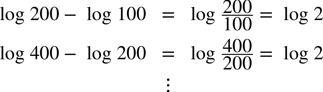
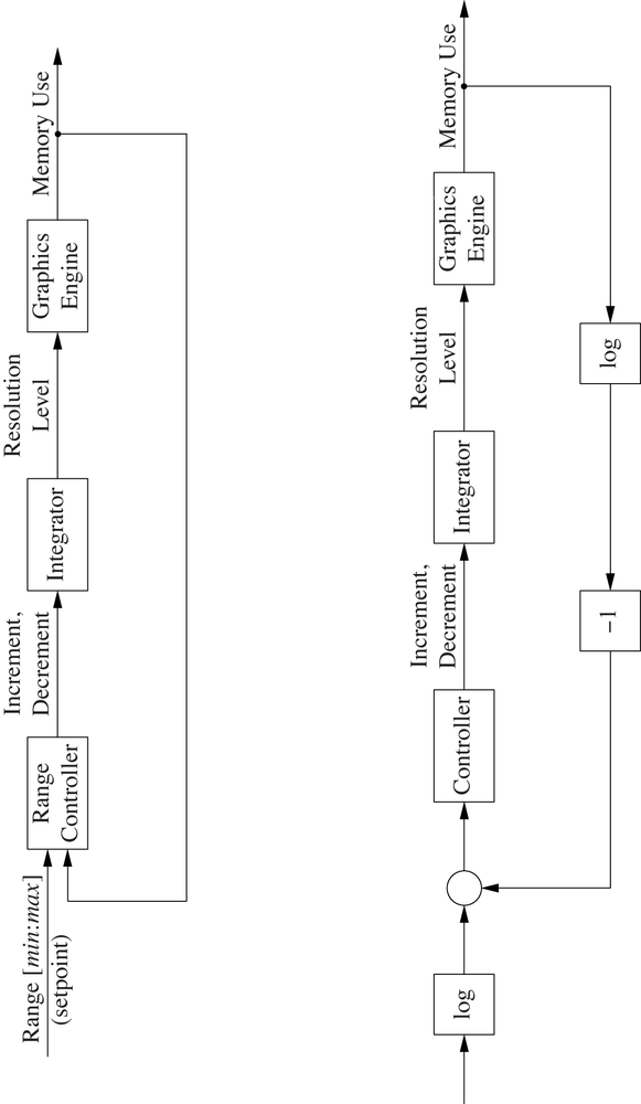
For this reason, we will use the logarithm of the memory consumption and the setpoint when we calculate the tracking error.

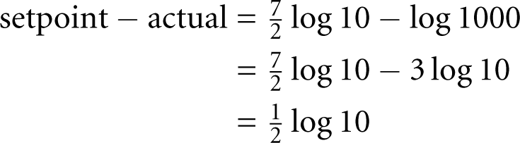
Using this loop architecture, the permissible range is specified as fixed controller parameters when the controller is first set up. Our requirements are that the controller should produce a nonzero output if memory consumption exceeds (say) 10,000 units. We will also introduce a lower threshold: if memory falls below (say) 1,000 units, the resolution should be increased.

We now choose as “setpoint” the arithmetic middle between the two threshold values and make the dead zone equal to the distance between the thresholds. Keep in mind that we are working with logarithms, so the setpoint should be the mean of the logarithms:

To find the width of the dead zone, we perform a similar calculation. The “tracking error” is a difference between logarithms. At the lower threshold, this error is

At the upper threshold (that is, when the actual memory consumption equals 10,000), we find a tracking error of . Hence, the dead zone extends from to , symmetrically around the setpoint at . To give ourselves some additional margin, we can choose tighter bounds, of course, such as , for example.

Typical results are shown in Figure 18-3.^[20] Memory consumption increases with the number of game objects. As consumption exceeds the critical threshold, the resolution level is decremented with the consequence that the memory required drops sharply (in fact, it is cut in half). This is especially obvious in the second half of the simulation: the number of game objects increases steadily; however, whenever the total memory consumption approaches the upper threshold, the resolution level is reduced and with it the amount of memory consumed. Similarly, if the number of game objects becomes small, then the resolution level is increased accordingly.

Figure 18-3. Typical closed-loop performance. In general, the amount of memory consumed grows with the number of game objects. If the memory consumption approaches the upper threshold, then the resolution level is reduced, cutting the amount of occupied memory in half.

In the spirit of the simulation framework, the following code uses the loop architecture based on a scalar setpoint (Figure 18-2, bottom). It is not difficult, however, to adapt the code to follow the nonstandard architecture in Figure 18-2 (top).

The simulation code describes a system with deterministic memory usage, but it is easy to add further sources of randomness. The controlled system itself is described by the class GameEngine. At each time step, there is a possibility that the number of game objects will change by 1 (in either direction). The total number of game objects must fall between 1 and 50.

import math
import random
import feedback as fb

class GameEngine( fb.Component ):
    def __init__( self ):
        self.n = 0    # Number of game objects
        self.t = 0    # Steps since last change

        # for each level: memory per game obj
        self.resolutions = [ 100, 200, 400, 800, 1600 ]

    def work( self, u ):
        self.t += 1

        # 1 change every 10 steps on avg
        if self.t > random.expovariate( 0.1 ):
            self.t = 0
            self.n += random.choice( [-1,1] )
            self.n = max( 1, min( self.n, 50 ) ) # 1 <= n <= 50

        crr = self.resolutions[u] # current resolution
        return crr*self.n         # current memory consumption

    def monitoring( self ):
        return "%d" % (self.n,)

In addition to the game engine, we need several other components to complete the control loop: the controller itself, the aggregator or actuator (called ConstrainingIntegrator in the code because it also constrains its output to the range of legal resolution levels), and finally an element to calculate the logarithm of the output signal.

class DeadzoneController( fb.Component ):
    def __init__( self, deadzone ):
        self.deadzone = deadzone

    def work( self, u ):
        if abs( u ) < self.deadzone:
            return 0

        if u < 0: return -1
        else:     return 1


class ConstrainingIntegrator( fb.Component ):
    def __init__( self ):
        self.state = 0

    def work( self, u ):
        self.state += u
        self.state = max(0, min( self.state, 4 )) # Allow 0..4
        return self.state


class Logarithm( fb.Component ):
    def work( self, u ):
        if u <= 0: return 0
        return math.log(u)

With all these components in place, we need only define a function to provide the setpoint; we can then complete the closed-loop operation in a single call.

fb.DT = 1

def setpoint(t):
    return 3.5*math.log( 10.0 )

c = DeadzoneController( 0.5*math.log(8.0) ) # width of deadzone
p = GameEngine()

fb.closed_loop( setpoint,c,p,actuator=ConstrainingIntegrator(),
                returnfilter=Logarithm() )