
Chapter 9. PID Tuning
Although the functional form of a PID controller is fixed, the gain parameters kp, ki, and kd are initially undetermined. To obtain a concrete implementation, we must select values for these parameters. At the same time, we are free to choose values that will lead to the most desirable behavior, given the situation and our objectives.
Finding appropriate values for the controller gains (“tuning” the controller) can be a frustrating exercise:[9] with two (for a PI controller) or even three (for a PID controller) parameters, the number of possible combinations to try out is very large. Moreover, it is often difficult to predict intuitively what effect an increase or decrease of any one of the parameters will have on the performance of the entire feedback loop. Some sort of guidance is therefore highly desirable.
If a good analytical model of the process is available, then root locus techniques (Chapter 24) can be extremely helpful. But if no analytical expression for the transfer function is known, then we must resort to measuring the dynamic response of the system and base our tuning strategy on the experimental results. The Ziegler–Nichols rules are a classic set of heuristics that require only a little information about the process. We can go a step further and first “fit” a phenomenological transfer function model to the experimental data (Chapter 8). That model is then used to derive suitable values for the controller gains analytically. Methods taking this approach include the Cohen–Coon and the modern AMIGO methods.
Tuning Objectives
The first goal of controller tuning is stability—unless we can be sure that the system won’t blow up, nothing else matters much. Once we have established stability boundaries for the parameters, we can attempt to find the best values within those boundaries in order to achieve the desired performance of the overall, closed-loop system.
Control systems can be optimized for different behaviors depending on the specific situation. Generally, this involves making typical engineering trade-offs between different desirable properties: fast systems are more susceptible to noise and oscillatory behavior; systems that are sluggish may provide better steady-state accuracy and robustness.
The most important questions for the performance of the overall, closed-loop system are as follows.
Is a non-vanishing tracking error in the steady state acceptable? For the overall system, a persistent error in the steady state is usually not acceptable (suggesting the use of an integral term in the controller). However, a complex control system may contain subsystems for which quick responses are more important than tracking accuracy. (Integral terms tend to slow the response down.)
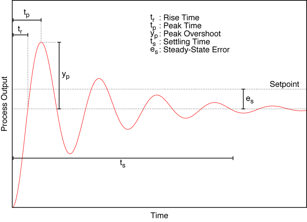
Is oscillatory behavior acceptable, and how quickly do the oscillations decay? Oscillatory behavior is often undesirable by itself (just imagine a car’s cruise-control system subjecting the passengers to such an experience). Furthermore, oscillatory systems necessarily overshoot the final settling value initially, which may be prohibited because it would violate some external constraint. That being said, oscillatory systems respond faster than overdamped systems.
How quickly does the system have to respond to input changes? The response time is determined by the duration of one period (for oscillatory systems) or by the time until the system reaches about two-thirds of its new steady-state value (for non-oscillatory systems). The system cannot respond faster than its dominant time scale.
Must the system be robust to noise? Noise is a high-frequency disturbance. To suppress its influence, the system needs to be relatively sluggish. This will often rule out derivative control, but it also requires longer response times overall. Systems that are robust to noise respond more slowly.
Specific performance requirements can be expressed in terms of various properties of the step response of the closed-loop system. For instance, we may require that the closed-loop system must have a “rise time” tr of less than 2.5 seconds to ensure sufficiently speedy response. (See Figure 9-1; the “settling time” is the time until the amplitude of the oscillations has fallen to less than 5 percent of the steady state.)
In addition to the customary requirements just enumerated, further questions may arise from time to time. For instance, if very high tracking accuracy is required, then a nested control loop (see Chapter 11) may be a good idea.
All the standard tuning “rules” (such as the Ziegler–Nichols and other methods discussed later in this chapter) make implicit choices about the desired accuracy and response time. These choices are intended to lead to acceptable performance for most practical applications, but they might well require augmentation on a case-by-case basis to deal with special situations.
General Effect of Changes to Controller Parameters
We can make some general statements about the typical effects that changes to the controller gains have on closed-loop performance. These observations can be useful when making manual adjustments to the values obtained from one of the systematic tuning methods described later in this chapter.
In general, increasing the controller gains leads to a speedier response but also tends to make the system less stable. This is not true for the derivative term: increasing the derivative gain leads to both greater speed and greater stability, provided that the signal is sufficiently free of noise. A nonzero integral gain is usually necessary to avoid a steady-state error (proportional droop, Chapter 4).
For a controller of the form
we can summarize the general rules as follows:
Increasing kp:
increases speed
decreases stability
enhances noise
Increasing ki:
decreases speed
decreases stability
reduces noise
eliminates steady-state errors more quickly
increases the tendency to oscillate
Increasing kd:
increases speed
increases stability
strongly enhances noise
These observations about the effects of changing the controller gains are often true, but not always. There are plants or processes that show different behavior—for example, one can find “conditionally stable” processes that become more stable when the proportional gain is increased in a closed-loop configuration.
Ziegler–Nichols Tuning
The Ziegler–Nichols tuning rules[10] for PID controllers are a set of simple heuristics intended to give adequate performance in a wide variety of situations. An essential aspect of Ziegler–Nichols tuning is that no knowledge of the plant’s transfer function is required: the rules are expressed entirely in terms the plant’s step-input response.
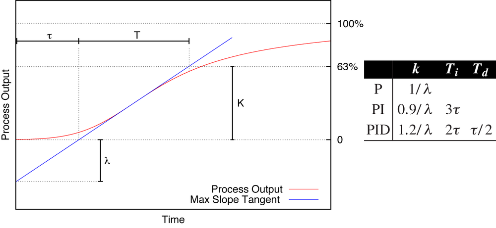
The Ziegler–Nichols rules are primarily intended for self-regulating processes, which eventually reach a steady state in response to a disturbance (Chapter 8). The method is similar to the one described in Chapter 8 to measure the dynamic response. Initially, the system is at rest, and then the response to a sudden setpoint change (in an open-loop configuration and without a controller) is observed. A tangent is fitted to the inflection point of the response curve (the point of greatest slope), and the intersection of the tangent line with the coordinate axes yields estimates for two parameters: τ and λ (see Figure 9-2).
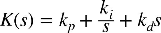
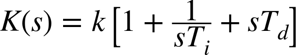
Once τ and λ are known, numerical values for the parameters in a PID controller can be found from the formulas included in Figure 9-2. Notice that Ziegler–Nichols rules are usually quoted in a way that assumes the controller K(s) is of the form
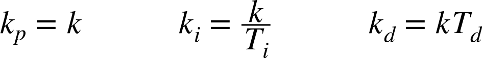
For controllers in the form K(s) = kp + ki/s + kds, it is necessary to use the following conversion formula:
The primary appeal of the Ziegler–Nichols method is its simplicity. The formulas for the controller gains are elementary, and the experimental procedure is simple and relatively fast. The reason is that it does not require the experiment to continue until the plant has reached its steady state—it is sufficient to wait until the curve exhibits an inflection point. However, the results will rarely be optimal, though they often turn out to be “good enough” in practice. Other times, they merely provide a starting point.
Semi-Analytical Tuning Methods
The Ziegler–Nichols rules are pure heuristics that were developed largely through empirical observations on real systems but without theoretical justification. A more analytical approach, which also utilizes more process information, involves first fitting a model to the step response and then moving the poles of the resulting transfer function to the desired locations (see Chapter 23). The resulting expression is then solved for the controller gains in terms of the model parameters. Because the models used for this purpose are sufficiently simple (in essence, they are the models we encountered in Chapter 8), one can express the result as closed formulas that require only “plugging in” of the experimental parameters.
Table 9-1 gives the results for two such methods—the classical Cohen– Coon method and the more modern AMIGO method.[11] Both methods employ the same model introduced in Chapter 8 to describe nonoscillatory self-regulating processes:

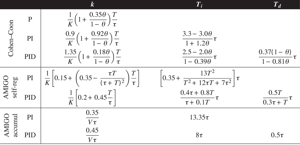
The AMIGO method also has a variant for accumulating processes, as described by the following model (also familiar from Chapter 8):

We must obtain values for K (or V), T, and τ from comparison with a step-response experiment as described earlier. The Cohen–Coon method uses the following dimensionless combinations of T and τ:

This quantity is sometimes known as the “controllability ratio.” For processes with a delay that is large compared to the process-internal time constant, θ approaches 1. Such processes are harder to control than processes with small θ.
Practical Aspects
The impressive appearance of the formulas in Table 9-1 should not obscure the fundamental limits of this approach. First of all, generic formulas cannot take problem-specific requirements into account. They were derived to achieve specific closed-loop performance characteristics, which may or may not provide the best balance of speed and stability for a particular application.
More importantly, these methods silently assume that the various parameters (K, V, T, and τ) can be observed with satisfactory accuracy (to within 1 percent for Cohen–Coon and AMIGO!). More often than not, this assumption is not justified in practice. Besides the obvious culprits (imperfect experimental setups, variations between experimental runs, and noise in the data), there is a more fundamental problem lurking here: the simple-lag-with-delay model underlying all these methods may not be particularly suitable for a given process. We saw in Chapter 8 that different models may fit the same data comparably well yet lead to quite different values for the parameters.
A particular concern is the “delay” parameter τ, since none of the methods give meaningful results if the observed delay vanishes. For industrial processes that have a lot of “inertia,” it is reasonable to expect that all responses are gradual and exhibit an apparent delay (as in Figure 9-2), but for other types of system the importance attached to τ seems overstated.
The practical advice is that, when given a set of experimental observations, try to make the best parameter estimates “in the spirit” of the methods described. Because the three methods make slightly different assumptions and attempt to optimize performance in slightly different ways, using all three to calculate controller gains will provide a range of numerical values over which one can expect reasonable performance of the closed-loop system. (In this context it is noteworthy that the Cohen–Coon method results are similar to those of the Ziegler–Nichols method for small θ.)
A Closer Look at Controller Tuning Formulas
Tuning methods such as the Ziegler–Nichols method and its relatives were developed using pole-placement methods (Chapter 23), primarily to describe industrial processes. It is interesting to take a closer, deconstructive look at the results in order to understand what’s going on—in particular with an eye to situations where the original assumptions are not valid.
If we plug the results of any one of the three methods presented here into the transfer function for the PID controller, we find that we can always write it in the following form (but do not confuse the controller’s transfer function K(s) with the process gain K):

with numerical coefficients α, β, and γ. Only the numerical values of the coefficients differ from method to method. Typically they fall into the following ranges:

For the Cohen–Coon and AMIGO methods, the factor C equals
![]() . For the Ziegler–Nichols method, the factor C equals
1/λ, where λ is the intersection of the tangent
with the vertical axis. But since the slope of the tangent is K/T and
since the tangent passes through 0 at τ, we can write
. For the Ziegler–Nichols method, the factor C equals
1/λ, where λ is the intersection of the tangent
with the vertical axis. But since the slope of the tangent is K/T and
since the tangent passes through 0 at τ, we can write ![]() as in the other two methods. Therefore, the factor C is
always
as in the other two methods. Therefore, the factor C is
always ![]() , even for the Ziegler–Nichols method.
, even for the Ziegler–Nichols method.
Finally, the process gain K is the ratio of the change in process output Δy that results from a change in control input Δu:

Pulling all the pieces together, we can write the controller’s transfer function as
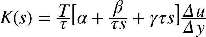
This result makes imminent sense. The rightmost factor Δu/Δy captures the static behavior of the plant: how much the input u needs to change in order to bring about a desired change in output y. When acting on a tracking error e, this factor will yield the change in input required to bring about a static change in output that equals e in magnitude.
The rest of the transfer function consists of adjustments—to the size of the control action—that take the system’s dynamic, time-dependent behavior into account. The leftmost factor T/τ measures to what extent the dynamics are dominated by lags or delays. Here it is helpful to adopt a broader notion of T and τ than “intersections on a graph.” Namely, the “delay” τ is the time duration until a change in input first becomes visible in the output. The “time constant” T is the time it takes for a change to fully take effect. The factor T/τ informs us that a sluggish system requires stronger actions: if it takes twice as long for a control action to fully take effect, then we must apply twice as large a correction to achieve the same effect in the same time.
We can say this differently: when acting on an error e, the term
![]() yields the control action u required to bring about a
change in process output that would cancel
e—provided the plant responds completely within
the next time step. But since the plant response is stretched over a duration
T, the control action needs to be increased by the same factor in order
to bring about an error-canceling response in the next time step.
yields the control action u required to bring about a
change in process output that would cancel
e—provided the plant responds completely within
the next time step. But since the plant response is stretched over a duration
T, the control action needs to be increased by the same factor in order
to bring about an error-canceling response in the next time step.
Conversely, if the delay doubles before an input change is visible in the output, then we must apply only half the correction because we will be applying it for twice as long (before the effect becomes visible).
Finally, the central term in brackets contains adjustments that are specific to each term in the PID controller. We find that the integral term is reduced by the apparent “delay” τ, which makes sense when one considers that the cumulative error has a tendency to build up during the time that a tracking error persists.
[9] Some studies have found that over 95 percent of industrially installed controllers are of the PID type—and that 80 percent of them function poorly, often because of improper tuning.
[10] This section describes the step-response variant of the Ziegler–Nichols method; there is also the so-called frequency-response variant. When using the frequency technique, integral and derivative controls are disabled and then the controller gain is increased “until the system begins to exhibit sustained, stable oscillations.” The controller gain values are then expressed in terms of the frequency and gain of this oscillation. Although important for electrical devices, it is hard to see how this method can be applied to general processes.
[11] The formulas given here follow the presentation of Advanced PID Control by Karl J. Ångström and Tore Hägglund (2005).