
Chapter 8. Measuring the Transfer Function
If we have a good theoretical model for the system under consideration, then we can derive the transfer function directly from the model by calculating the Laplace transform of the differential equation that describes the system dynamics. More often than not, however, there won’t be a good analytical model. In those cases, we will have to measure the transfer function in a process known as system identification. Even if we have a good model, we will still need to perform some measurements to “fit” the model’s parameters.
There are basically two different questions we need to ask.
These are the basic questions we want to answer through observations. The answer to the first one is captured in the static process characteristic, the answer to the second in the dynamic process reaction curve or plant signature.
All measurements are done in an open-loop arrangement, and without a controller:

In that way, we can adjust the input in an arbitrary fashion as desired, so that we observe only the response of the system or plant alone.
Static Input/Output Relation: The Process Characteristic
The static process characteristic provides us with some basic but essential information. Obtaining it seems simple enough: apply a steady input value, wait until the system has settled down, and record the output. A typical graph might look like the one in Figure 8-1. There is a minimal control input that is required to bring about any change, and for large inputs the system begins to saturate and no longer follows the input faithfully.

The most important feature of this curve is its local slope, which in this context is also known as the process gain. Specifically:
The magnitude of the process gain provides information about the size or strength of the control actions that will be needed to bring about significant change in process output.
The sign of the process gain provides information about the directionality of the input/output relation; if it is positive, then a regular control loop will work. But if the process gain is negative, then we must use an inverted loop arrangement (see Chapter 5).
If the process gain undergoes drastic change over the typical operating range (so that control actions of different strength are needed to bring about comparable change for different input values), then the system is harder to control and we may need to consider gain scheduling (see Chapter 11).
Ideally, we’ll be able to operate our system in the linear region, where the process output is more or less proportional to the control input (as indicated in Figure 8-1).
Practical Considerations
The simple description of the measurement process omits several practical considerations.
How long should we wait—after making the input change—for the system to reach its new steady state, so that we can take our measurement?
Will the system reach a steady state at all, or will the output keep growing unless stopped? (The cache hit rate is an example for a self-regulating process that naturally reaches a steady state. The opposite is an accumulating process, such as water flowing into a tank: once the input valve is open, the level in the tank will continue to increase.)
How repeatable are the measurements? If we run the same experiment multiple times, how much difference is there in the observed outputs? (This is a measure for the amount of noise in the system.)
If we perform the experiment with input values increasing from data point to data point, and then run it again with input values decreasing, do we find the same results? If not, this is a sign of hysteresis in the plant.
Will we even be able to perform extensive experimentation? On production systems, it may not be possible to change the control input in a random fashion.
We can see that, in many cases, circumstances are such that we will have to make do with very small data sets indeed—possibly consisting of just a handful of points. (In Chapter 14, we will discuss a system where each data point requires a full day before a measurement can be taken.)
Nevertheless, we must be sure to obtain the two crucial bits of information about the process: the sign of the process gain and an approximate estimate for its magnitude. Without those bits of knowledge, we can’t proceed.
Dynamic Response to a Step Input: The Process Reaction Curve
To measure the dynamic response, all we really have to do is switch the system on and see what happens! The system should be at rest initially (with zero input). We then apply a sudden input change and record the development of the output value over time. To obtain a good signal-to-noise ratio, the input step should be large—and we should probably repeat the whole process a few times with different input amplitudes. (Remember that this is done on the plant alone, without feedback and without a controller.)
It is possible in theory to extract all information about the transfer function from the step response, but in practice we are usually most interested in just a few essential parameters. For us, the following three are the most important (compare Figure 8-2).
- Process gain K:
This is the ratio between the value of the applied input signal and the value of the final, steady-state process output after all transients have disappeared. If the process is in the proportional range, then the process gain will be independent of the input value (thus, an input signal that is twice as large will lead to an output that it also twice as large).
- Time constant T:
The time it takes for the process to settle to a new steady state after experiencing a disturbance. The time constant is usually defined as the time it takes the process to reach about two thirds (or 1 – exp(–1) ≈ 0.63) of its final value. (The process output approaches the steady state asymptotically, so in principle the time required to reach 100 percent of the final value is infinite.)
- Dead time τ:
Some processes exhibit a measurable delay until an input change begins to affect the output. In physical systems, such delays are usually due to transport phenomena (like liquid flowing through a pipe, or heat through a conductor, before reaching a sensor).
Some important tuning methods are based on those parameters alone (see Chapter 9).
Practical Aspects
Similar considerations apply in the case of experiments to determine the dynamic response as when attempting to obtain the static process characteristic, as discussed previously. In particular, we must be able to apply a step input in a controlled fashion and then prevent any further changes in input until the system has reached its steady state. In the case of accumulating processes that do not settle to a steady state, we must decide how long we can run them before exceeding the system’s buffering capacity.
The primary reason for running experiments of this kind is to obtain enough information for controller tuning. In Chapter 9, we will discuss the Ziegler–Nichols tuning method, which attempts to make do with only minimal process knowledge.
Process Models
We can also attempt to formulate an analytical model for the transfer function and then “fit” it to the data obtained from the step-input experiment (also known as a “bump test”). In the absence of knowledge about the process internals, we will choose models that are both simple and convenient and also do a reasonable job of replicating the observed behavior. These models tend to be parameterized by the same three basic quantities already introduced: process gain K, time constant T, and delay τ. Such models are, of course, only phenomenological; their predictions need to be taken with a grain of salt, since they are not justified by any theoretical arguments. (If we have knowledge about the process internals, then we should of course take it into account when formulating a model.) Examples of some of the most frequently encountered behaviors are discussed next.
Self-Regulating Process
This is the easiest case: in response to a step-like input, the system simply approaches the steady state, possibly after a delay, but without overshoot or oscillations (see Figure 8-2). Because they eventually settle to a steady state, such processes are called self-regulating.

One can obtain a rough estimate for the three parameters by using the geometric construction shown in Figure 8-2, where a tangent is drawn through the inflection point (the point with greatest slope) of the process reaction curve. The intersections of this tangent line with y = 0 and y = 0.63 are then used to determine the two time scales τ and T. The process gain K is found from the value of the process output in the long-time limit (divided by the amplitude of the input step change).
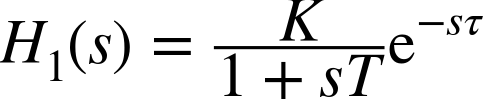
Alternatively, one can estimate the parameters by fitting an appropriate model. The following model (in the time domain) is often used to describe the step response for this type of process (see Figure 8-3):

where τ is the dead time and T is the time constant. This model is chosen mainly because it has a particularly simple transfer function in the frequency domain:[6]
One problem with this model is that the slope of f1(t) does not vanish as t → τ. So instead we can use the following, more complex model for the step response that displays a little “foot” for small t (see Figure 8-3):
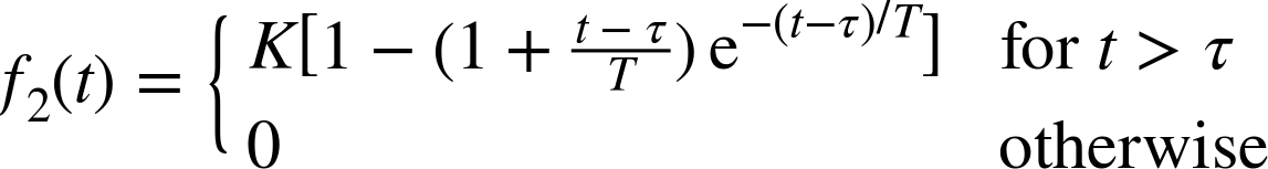
Although it is more complex in the time domain, in the frequency domain this model is still fairly simple:
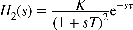
Figure 8-3 shows the step response for both models. At first it may appear as if the two models are really rather different, but by changing the parameters T and τ the two models can be made to look quite similar. The figure shows both f1(t) and f2(t) with the parameter values T = 1 and τ = 2, as well as the simple model f1(t) but with parameters T = 1.67 and τ = 2.53 (indicated as f1*(t) in the figure). With this choice of values, the simple model f1(t) begins to look very much like the more complex model f2(t), except for a short time at the beginning.

We should take two things away from this exercise. Unless we have good reasons to choose a more complicated model, we might as well stay with a simple one, since it is (within experimental accuracy) likely to be almost as good a description of the process as a more complex one. Furthermore, we should not put too much weight on the “fitted” parameter values obtained in this way, since a seemingly small change in model can lead to rather significant changes in parameter values.
Accumulating Process
For integrating or accumulating processes, the step-input response does not settle to a steady state; instead, it continues to increase. This type of process primarily describes queueing situations and other scenarios where incoming items “pile up” until they are being handled. The models from the previous section are obviously not suitable, so a different model is needed (see Figure 8-4).

We can again formulate a model that uses three parameters—namely, the velocity gain or integrating gain V, the time constant T, and the delay τ. Time constant and delay are familiar from before, but the velocity gain V must not be confused with the static gain K. The velocity gain V is a measure of the final growth in output, and we can obtain it from the slope of the asymptote (as shown in Figure 8-4). Accordingly, its dimension is process output over time. (In contrast, the gain K is a measure of the final process output itself and has the same dimension as the output signal.)

In the frequency domain, this model has the form

The most important feature of accumulating processes is, of course, the asymptotic growth in process output. Hence we can often neglect the internal dynamics, which are determined by T. This leads to a simplified model (see Figure 8-5) with the following step response in the time domain:
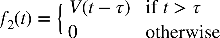

The model itself has the following transfer function in the frequency domain:

The delay τ is the time after the step input at which the process output first becomes nonzero. (Of course, the delay may be zero.) The velocity gain V must be determined from the slope of the curve, as shown in the figure.
Self-Regulating Process with Oscillation
Many mechanical or electrical devices exhibit a behavior that is more complicated than the ones just discussed. Such systems do not simply approach a new steady state value in response to an external disturbance but rather exhibit damped oscillations. In other words, in response to a step input, they overshoot the final value initially and then continue to oscillate around it for some time (see Figure 8-6). Think of a mass on a spring whose free end is suddenly moved to a different position: unless its motion is restricted (by being submerged in honey or otherwise damped), the mass will not just creep to its new position; it will begin to oscillate.

A common step-response model exhibiting oscillations is

with the frequency domain representation
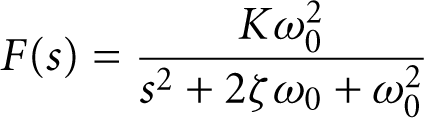
Here ω0 is the natural frequency of the system, ζ is the damping factor (controlling how quickly the amplitude of the oscillations diminishes), and ![]() is the frequency of the damped oscillations.
is the frequency of the damped oscillations.
Although extremely common among mechanical and electrical devices, this process model is rare in computer systems or industrial processes.[7]
Non-Minimum Phase System
Systems with this ungainly name have the perverse characteristic that their initial response to a control input is in the opposite direction from the input! (See Figure 8-7.)

This is not as far-fetched as it may sound. For instance, think of a compute server, where the input is the number of active CPU instances and the output is the average query response time. If the process of activating additional CPUs takes cycles away from the already active CPUs, then the query response time will suffer while those new CPUs are being activated. More generally, this kind of behavior can occur whenever the system incorporates two distinct processes (with different time constants) that move the output in opposite directions. Systems exhibiting this kind of inverse response are difficult to control and require special techniques.
Other Methods of System Identification
The appeal of step input methods is their simplicity. For situations where we have a need for higher accuracy (and where we have additional understanding of the system dynamics), there are other, more accurate, methods. For example, rather than applying a step input, we can (at least in principle) apply a sinusoidal input signal. If the system under investigation is, in fact, linear, then its output to such an input will also have the shape of a sine wave with the same frequency but perhaps with a different amplitude and phase. We would therefore apply a sine input with a given frequency, wait until all transient behavior has died away, and then compare the amplitude and phase of the input and the output. This process is repeated for a variety of (input) frequencies and then plotted in a Bode plot (see Chapter 25).
This method has great theoretical appeal but can be difficult to apply outside the electronics lab, mostly because it is time consuming. For each of the (many) frequencies that need to be tried, one must wait until all transients have disappeared before making a measurement. This does not matter much if transients disappear in seconds, but if the typical time scale of the process is measured in minutes or hours then the process will clearly become very tedious. It may also not be feasible to generate a sinusoidal input signal for a real-world process.
Still another set of methods is based on correlation functions. An input signal is applied, and the correlation function between the input signal and the output signal is calculated. From this information, the system’s transfer function can be calculated.[8]
[6] To find the step response, multiply the transfer function H(s) by the frequency representation of the unit step, which is 1/s, and then transform the resulting expression back into the time domain. See Chapter 20 for a worked example.
[7] The details are discussed in every book on control theory. See Appendix D for some suggestions.
[8] The details are far beyond the scope of this book. Some accessible information can be found in The Art of Control Engineering by K. Dutton, et al. (1997).