The situation sketched in the paragraph above is common enough, but it can describe quite a variety of circumstances, depending on the specifics. Details matter! For now, we will assume the following.

This set of conditions defines a specific, concrete control problem. From the control perspective, the absence of any accumulation of pending requests (no queueing) is particularly important. Recall that a queue constitutes a form of “memory” and that memory leads to more complicated dynamics. In this sense, the case described here is relatively benign.

The description of the available information already implies a choice of output variable: we will use the “success ratio,” which is the ratio of answered to incoming requests. And naturally we will want this quantity to be large (that is, to approach a success rate of 100 percent). The number of active servers will be the control input variable.

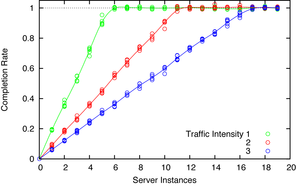
Obtaining the static process characteristic is straightforward, and the results are not surprising (see Figure 15-1): the success rate with which requests are handled is proportional to the number of servers.^[16] Eventually, it saturates when there are enough servers online to handle all requests. The slope and the saturation point both depend on the traffic intensity.

In regards to the dynamic process reaction curve, we find that the system responds without exhibiting a partial response. If we request n servers then we will get n servers, possibly after some delay. But we will not find a partial response (such as n/4 servers at first, n/2 a little later, and so on). This is in contrast to the behavior of a heated pot: if we turn on the heat, the temperature begins to increase immediately yet reaches its final value only gradually. Computer systems are different.

We can obtain values for the controller parameters using a method similar to the one used in Chapter 14: the tuning formulas (Chapter 9) consist of the static gain factor Δu/Δy multiplied by a term that depends on the system’s dynamics. Because in the present case the system has no nontrivial dynamics, we are left with the gain factor. From the process characteristic (Figure 15-1), we find that

for intermediate traffic intensity. Taking into account the numerical coefficients for each term in the PID controller, we may choose

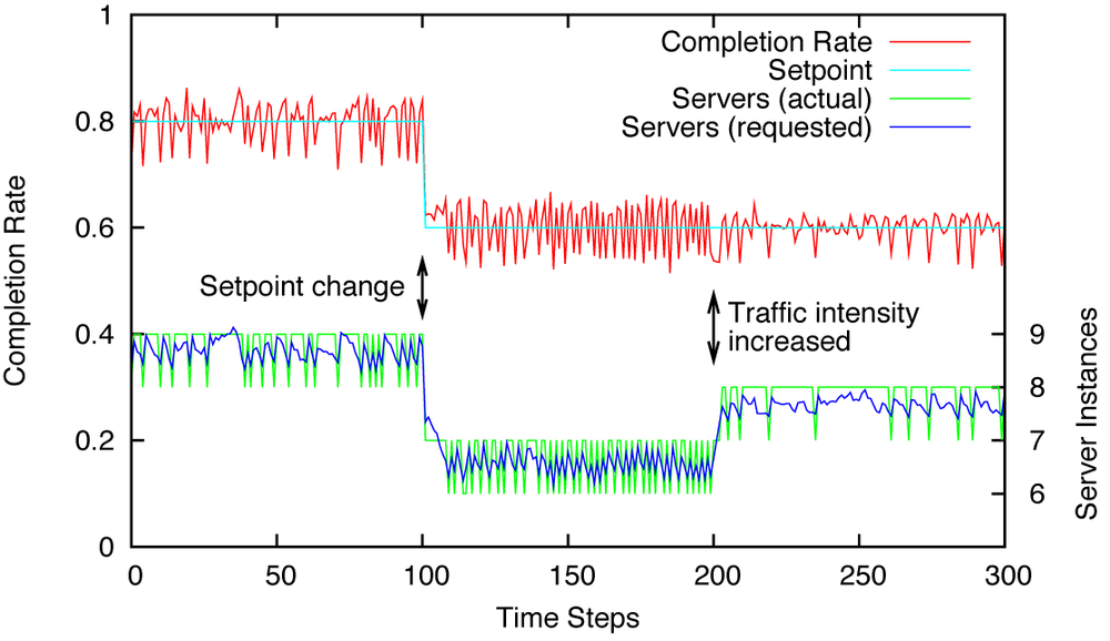
as controller gains. Figure 15-2 shows the resulting behavior for setpoint values much less than 100 percent. The system responds nicely to changes in both setpoint and load.

Figure 15-1. The steady-state relationship between the completion rate and the number of server instances (the static process characteristic).

The system is very oscillatory, but in this case this is not due to a badly tuned controller, but to the inability of the system to respond accurately to its control input. This is especially evident in the middle section of the right-hand graph in Figure 15-2 (between time steps 100 and 200): six server instances are clearly not enough to maintain the desired completion rate of 0.6, but seven server instances are too many. Because we can’t have “half a server,” the system will oscillate between the two most suitable values.

Figure 15-2. Closed-loop behavior when using a PID controller and desired completion rates that do not approach 100 percent.

A success rate of 80 or even 90 percent is not likely to be considered sufficient—ultimately, we want to reach a state where there are just enough servers to handle all requests. This will require a modification of the usual approach as well as a nonstandard (nonlinear) controller.

We begin by choosing a high setpoint, something on the order of 0.999 or 0.9995. In practice, we will not be able to track this setpoint very accurately. Instead, we will often observe a 100 percent completion rate simply because the number of servers sufficient to answer 999 out of 1,000 requests has enough spare capacity to handle one more. This is a consequence of the fact that we can add or remove only entire server instances, and would occur even if there was no noise in the system.

It is important that the setpoint is not equal to 1.00. The goal of achieving 100 percent completion rate is natural, but it undermines the feedback principle. For feedback to work, it is necessary that the tracking error can be positive and negative. With a setpoint value of 1.00, the tracking error cannot be negative:

and this removes the pressure on the system to adapt. (After all, it is easy enough to achieve a 100 percent completion rate: just keep adding servers. But that’s not the behavior we want.)

As long as the setpoint is less than 1.00, an actual completion rate of 100 percent results in a finite, negative tracking error. This error accumulates in the integral term of the controller. Over time, the integral term will be sufficiently negative to make the system reduce the number of instances. This forces the system to “try out” what it would be like to run with fewer instances. If the smaller number of servers is not sufficient, then the completion rate will fall below the setpoint and the number of servers will increase again. But if the completion rate can be maintained even with the lower number of servers (because the number of incoming requests has shrunk, for instance), then we will have been able to reduce the number of active servers.

But now we face an unusual asymmetry because the tracking error can become much more positive than it can become negative. The actual completion rate can never be larger than 1.0, and with a setpoint of (say) r = 0.999, this limits the tracking error on the negative side to 0.999 – 1.0 = –0.001. On the positive side, in contrast, the tracking error can become as large as 0.999, which is more than two orders of magnitude larger. Since control actions in a PID controller are proportional to the error, this implies that control actions that tend to increase the number of servers are usually two orders of magnitude greater than those that try to decrease it. That’s clearly not desirable.

We can attempt various ad hoc schemes in order to make a PID-style controller work for this system. For instance, we could use different gains for positive and negative errors, thus compensating for the different range in error values (see Figure 15-3). But it is better to make a clear break and to recognize that this situation calls for a different control strategy.

Fortunately, the discussion so far already contains all the needed ingredients—we just need to put them together properly. Two crucial observations are:

These two observations suggest the following simple control strategy:

Step 4 is crucial: it is only through this periodic reduction in the number of servers that the system responds to decreases in request traffic. We can make the controller even more responsive by scheduling trial steps more frequently after a decrease in server instances than after an increase.

Figure 15-3. Choosing a high setpoint (such as r = 0.9995) is a problem because the tracking error can become much more positive than it can become negative. Here we use a controller that uses different gains for negative and positive tracking errors.

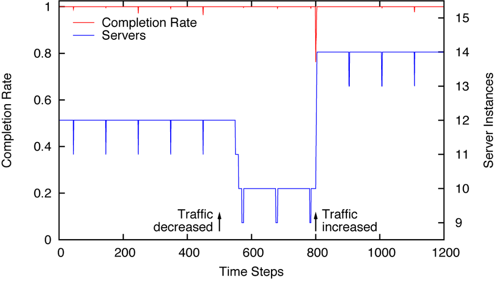
Figure 15-4 shows typical results, including the response to both a decrease and an increase in incoming traffic. The operation is very stable and adjusts quickly to changes. Another benefit (compared to the behavior shown in Figure 15-3) is that the system oscillates far less. The number of server instances is constant, except for the periodically scheduled “tests.”

Figure 15-4. Much better results can be obtained using a special controller that increases or decreases the number of server instances based only on the sign, not the magnitude, of the tracking error. (See main text for details.)

Until now we have assumed that any new server instances would be available immediately, one time step after the request. In practice, this is not likely to be the case: spinning up new instances usually takes a while, maybe a couple of minutes. Because the interval between control actions is on the order of seconds, this constitutes a delay of two orders of magnitude! That is too much time to ignore.

When it comes to latency, textbooks on control theory usually recommend that one “redesign the system to avoid the delays.” This may seem like unhelpful advice, but it is worth taking seriously. It may be worth spending significant effort on a redesign, because the alternatives (such as the “Smith predictor”; see Chapter 11) can easily be even more complicated.

In the present situation, one way to deal with the latency issue is the introduction of a set of “warm standbys” together with a second feedback loop that controls them (see Figure 15-5). There must already be a network switch or router present, which serves as a load balancer and distributes incoming requests to the various server instances. This switch should be able to add or remove connections to server instances very quickly. As long as we always have a sufficient number of spun-up yet inactive server instances standing by, we can fulfill requests for additional resources as quickly as the router can open those connections (quite possibly within one or two time steps).

Figure 15-5. A possible control architecture to deal with latency in spinning up additional server instances. A “fast” loop controls the number of instances currently active, based on the rate at which requests are completed; a “slow” loop maintains a pool of warm standbys.

In addition, we will need a second control loop that regulates the number of available standbys. We must decide how many standbys we will need in order to maintain our desired quality of service in the face of changing traffic patterns: that will be the setpoint. The controller in this loop simply commissions or decommissions server instances in order to maintain the desired number of reserves. This second loop will act more slowly than the first; its primary time scale is the time it takes to spin up a new instance. In fact, we can even set the sampling interval for this second loop to be equal to the time it takes to spin up a new server. With this choice of sampling interval, new instances are again available “immediately”—the delay has disappeared. (There is no benefit in sampling faster than the system can respond.)

The system that we want to simulate is a server farm responding to incoming requests. We must decide how we want to model the incoming requests. One way would be to create an event-based simulation in which individual requests are scheduled to occur at specific, random moments in time. The simulation then proceeds by always picking the next scheduled event from the queue and handling it. In this programming model, control actions need to be scheduled as events and placed onto the queue in the same way as requests.

We will use a simpler method. Instead of handling individual requests, we model incoming traffic simply as an aggregate “load” that arrives between control actions. Each server instance, in turn, does some random amount of “work,” thereby reducing the “load.” If the entire “load” is consumed in this fashion, then the completion rate is 100 percent; otherwise, the completion rate is the ratio calculated as the completed “work” divided by the original “load.”

The implementation is split into two classes, an abstract base class and the actual ServerPool implementation class. (This design allows us to reuse the base class in Chapter 16.)

import math
import random
import feedback as fb

class AbstractServerPool( fb.Component ):
    def __init__( self, n, server, load ):
        self.n = n           # number of server instances
        self.queue = 0       # number of items in queue

        self.server = server # server work function
        self.load = load     # queue-loading work function


    def work( self, u ):
        self.n = max(0, int(round(u))) # server count:
                                       # non-negative integer

        completed = 0
        for _ in range(self.n):
            completed += self.server() # each server does some
                                       # amount of work

            if completed >= self.queue:
                completed = self.queue # "trim" to queue length
                break                  # stop if queue is empty

        self.queue -= completed        # reduce queue by work
                                       # completed

        return completed


    def monitoring( self ):
        return "%d %d" % ( self.n, self.queue )


class ServerPool( AbstractServerPool ):
    def work( self, u ):
        load = self.load()        # additions to the queue
        self.queue = load         # new load replaces old load

        if load == 0: return 1    # no work:
                                  # 100 percent completion rate

        completed = AbstractServerPool.work( self, u )

        return completed/load     # completion rate

When instantiating a ServerPool, we need to specify two functions. The first is called once per time step to place a “load” onto the queue; the second function is called once for each server instance to remove the amount of “work” that this server instance has performed. Both the load and the work are modeled as random quantities, the load as a Gaussian, and the work as a Beta variate. (The reason for the latter choice is that it is guaranteed to be positive yet bounded: every server does some amount of work, but the amount that each can do is finite. Of course, other choices—such as a uniform distribution—are entirely possible.) The default implementations for these functions are:

def load_queue():
    return random.gauss( 1000, 5 )     # default implementation

def consume_queue():
    # For the beta distribution : mean: a/(a+b); var: ~b/a^2
    a, b = 20, 2
    return 100*random.betavariate( a, b )

Figure 15-4 shows the behavior that is obtained using a special controller. This controller is intended to be used with a setpoint of, so that the tracking error (which is also the controller input) can never be negative. When the input to the controller is positive, the controller returns, thus increasing the number of server instances by 1. When the input is zero, the controller periodically returns –1, thereby reducing the number of server instances.

The controller uses different periods depending on whether the previous action was an increase or a decrease in the number of servers. The reason is that any increase in server instances is always driven by a positive tracking error and can therefore happen over consecutive time steps. However, a decrease in servers is possible only through periodic reductions—using a shorter period after a preceding reduction makes it possible to react to large reductions in request traffic more quickly.

class SpecialController( fb.Component ):
    def __init__( self, period1, period2 ):
        self.period1 = period1
        self.period2 = period2
        self.t = 0

    def work( self, u ):
        if u > 0:
            self.t = self.period1
            return +1

        self.t -= 1        # At this point: u <= 0 guaranteed!

        if self.t == 0:
            self.t = self.period2
            return -1

        return 0

The controller is an incremental controller, which means that it does not keep track of the number of server instances currently online. As an incremental controller, it computes and returns only the change in the number of server instances. We therefore need to place an integrator between the controller and the actual plant in order to “remember” the current number of server instances and to adjust it based on the instructions coming from the controller:

To simulate a closed loop using this controller is now simple:

def setpoint( t ):
    return 1.0

fb.DT = 1

p = ServerPool( 0, consume_queue, load_queue )
c = SpecialController( 100, 10 )
fb.closed_loop( setpoint, c, p, actuator=fb.Integrator() )