In Chapter 20, we saw that, in the frequency domain, a system’s dynamic response y(s) to an external input u(s) is given by the product of the system’s transfer function H(s) and the input^[22]

We can express this equation as a block diagram, where the system (described by its transfer function H) transforms the input u to the output y:

Obviously, we can combine several such systems in series, with the output of one serving as input to the next:

The output of this composite system is the product of its components:

This follows simply because the output of the first element is x(s) = G(s) u(s) and because the output of the second component, acting on the output of the first, is y(s) = H(s) x(s). Therefore, the transfer function of the aggregate system consisting of H(s) and G(s) arranged in series is the product of the components: T(s) = H(s) G(s) = G(s) H(s). (Because G and H are merely functions, they commute.)

By similar reasoning, one can show that if two components are arranged in parallel,

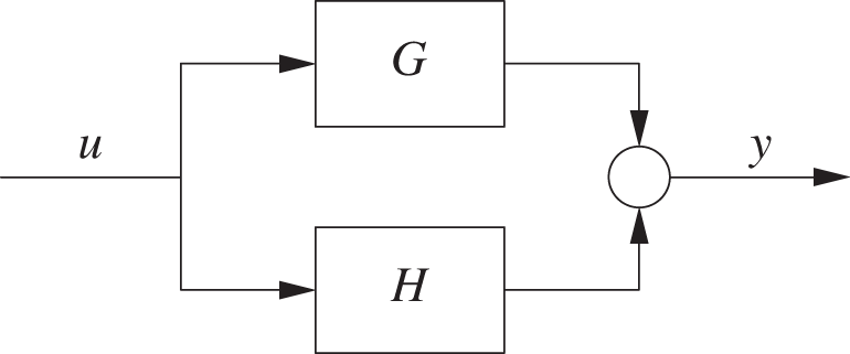
then one can add their respective outputs to find the output of the overall system:

The transfer function of a composite system, consisting of H(s) and G(s) arranged in parallel is the sum of the components: T(s) = H(s) + G(s).

These two simple rules allow us to handle a variety of open-loop systems. But we also need a rule for closed-loop arrangements. This will lead to a central result in the theory of feedback systems.

Suppose now that we have a desired outcome (a setpoint) for the system. In other words, we want the system outcome y to track a given reference signal r as closely as possible. To ensure this behavior, we apply the feedback principle (Chapter 2):

In other words, if y exceeds r, then we will adjust the input u in such a way that y will be reduced, and vice versa.

Toward this end, we “close the loop” so that the output y can be compared to the setpoint r (see Figure 21-1). All inputs to the circle are summed, and the result is then passed to the controller K. Because the system output y has been multiplied by –1 on its return path, the input to K is the tracking error e = r – y. We wish to minimize the magnitude of this error (in other words, we want to reduce it to zero). The controller K transforms the tracking error into a control input u to the system; when the tracking error is zero, no further changes need to be made to the input.

Figure 21-1. The standard feedback loop. The controller K acts on the tracking error e to produce the input u for the plant H. The plant output y is multiplied by –1 on the return path. At the circle, the negative output –y is added to the setpoint r to yield the tracking error e = r – y.

By construction, the system H transforms an input u into an output y. We may now treat the whole assembly as a single system (pictured in Figure 21-1 by the dashed box) that transforms the input r into an output y. What is the correct expression describing the behavior of this closed-loop system in terms of its components K and H? It can’t simply be the open-loop expression y = HK r, which fails to take into account that the output y is fed back into the system input. Instead, the combined system H K acts on the tracking error e = r – y to produce the output y:

Because H and K are regular functions, we can solve this equation for y. First multiply out the parentheses on the right-hand side,

and then bring the second term to the left-hand side:

Now factor out the common factor y on the left:

and finally divide by (1 + HK) to obtain

The transfer function of the closed-loop arrangement shown in Figure 21-1 is therefore

This result is central to all of feedback control theory.

An Alternative Derivation of the Feedback Equation

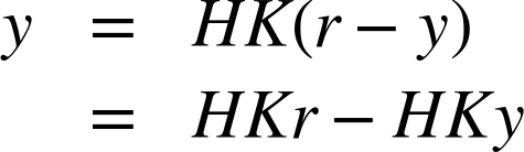
There is an instructive alternative to deriving the feedback equation, one that makes the iterative aspect of the feedback principle explicit. We begin once again with the basic input/output relation

y = HK(r – y)

but, instead of solving the equation algebraically, we take an iterative approach by plugging the expression y = HK (r – y) back into the equation on the right-hand side:

Now we do it again:

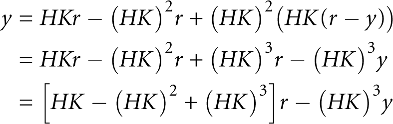
and so on. Writing it this way shows more clearly how the output y is being passed through the system HK again and again, and modified each time by the influence of HK. If HK has the effect of amplifying its input, then we can see that y will get large very quickly as it goes through the loop repeatedly.

Finally, summing the geometric series in HK will lead us back to the feedback formula. (That’s because x – x² + x³ – ⋯ = –x (1 – x + x² – ⋯) = x/(1 + x)—provided |x| < 1, for otherwise the sum does not converge. This condition provides yet another hint at the constraints that exist for the design of a suitable controller.)

Given the feedback equation that describes a closed-loop arrangement, we now have a set of “rules” that allows us to manipulate block diagrams and find the transfer function of a composite system directly from its block diagram. The rules are summarized in Figure 21-2.

These rules can be used to simplify complex block diagrams and also to modify existing ones. For instance, any series of elements H and G can be replaced by a single element with transfer function HG. Introducing an additional element (such as a filter F) into an existing loop merely amounts to the insertion of an additional factor into the transfer function for the entire loop, and so on.

One can formulate a wide variety of additional rules, but all can be reduced to the three basic rules given here. In any case, the rules shown in Figure 21-2 are sufficient for all block-diagram manipulations in this book.

Figure 21-2. The three most important operations of block-diagram algebra: composition in sequence (top), addition in parallel (center), and the negative feedback loop (bottom).

The transfer function technology described in the last two chapters may seem like magic: it turns differential equations into simple functions and allows us to manipulate entire control loops through a simple algebra of graphical operations! In the following chapters, we will see how this method allows us also to determine the dynamic response of closed-loop systems from the mathematical structure of the transfer function alone—that is, without actually having to evaluate any time-domain behavior.

That being said, transfer function methods are based on the Laplace transform and are applicable only when certain conditions are met:

There are techniques to extend transfer function methods to more general situations, and there is an alternative formulation of the theory that is not limited to single-input/single-output systems (see Chapter 26).

Beyond the direct applicability of Laplace transforms and transfer functions to performing calculations on specific systems, methods based on Laplace transforms provide a conceptual framework and—in many ways—the terminology for control systems. For this reason alone, it is necessary to gain at least a passing familiarity with them.