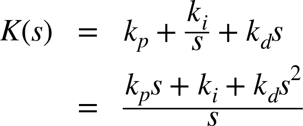
As we saw in Chapter 4, the output u_PID(t) of a PID controller in terms of its input e(t) is given by

Notice that u_PID(t) is linear in e(t). (Both integration and differentiation are linear operations.) The linearity of the PID controller is one reason for its popularity.

We can take the Laplace transform of this expression term by term to obtain the dynamic response of a PID controller in the frequency domain. Using Table 20-1, we find without difficulty that

The expression within brackets is the transfer function of the controller in frequency space. It has a particularly simple form—in fact, just the factors s and 1/s are often used to signify the corresponding terms (see Figure 22-1).

Figure 22-1. The standard form of the three-term or PID controller.

As we have just seen, the transfer function of a PID controller is

This is the form most convenient for theoretical work. It has the disadvantage that the three constants (k_p, k_i, and k_d) do not all have the same dimensions, because s has the dimension of frequency, k_i has the dimension of time, and k_d has the dimension of 1/time. In application-oriented contexts, an alternative form of the PID controller transfer function is often used:

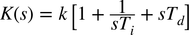
Here k is the controller gain, T_i is the “integral time” (or “reset time”), and T_d is the “derivative time” (or “rate time”). The two forms are equivalent, and the parameters are related:

Of course, the numerical values are different! When comparing values for controller parameters, one must not forget to establish which of the two forms they refer to.

The discussion so far has concerned only controllers that consist of strictly proportional, integral, and derivative terms (PID controllers). This raises the question of what else a controller can be. The answer is: anything at all, as long as it has one input and one output and depends only on values that are available at the time that control action is needed. If we want to use Laplace transforms and transfer function technology, then the controller behavior must be describable by a linear and time-invariant differential equation in the time domain. In principle, though, the controller action can be any function of its inputs.

If we were to start entirely from scratch, then what would the most desirable controller look like? Since our intent is for the plant output to track the setpoint signal as closely as possible, the “ideal” controller would act in such a way as to cancel the effect of the plant. Under those conditions, the input to the controller r would be precisely the output of the plant y (in an open-loop configuration):

Now assume that K exactly “neutralizes” or cancels the effect of H and so this equation becomes

Perfect tracking!

In frequency space, this is easy enough to achieve. Let H(s) be an arbitrary transfer function. Then a controller with the following transfer function will literally cancel the effect of the plant H:

All that remains to do is to transform this transfer function back into the time domain and then build a physical device that exhibits the required dynamical behavior. Of course, there is the rub: controller designs obtained in this way often require arbitrarily large control actions—larger than can be achieved using physical devices. This is not helpful. (But controllers that attempt to cancel the plant approximately are sometimes used as part of a global control strategy; recall the discussion of the Smith predictor in Chapter 11.)

The PID controller, together with a feedback architecture, takes a different approach: the controller does not attempt to cancel the plant dynamics exactly. Instead, it relies on frequent and continuous adjustments in order to have the plant output track the setpoint. For processes with difficult dynamics, however, a controller that is more complicated than a simple three-term controller may lead to better performance.

In Chapter 4, we mentioned the inability of a strictly proportional controller to track a setpoint without incurring a steady-state error. Now, with the controller’s transfer function and the feedback equation (Chapter 21) in hand, we can understand this phenomenon more precisely.

For a simple feedback loop with a plant H and a strictly proportional controller K = k, the feedback equation is

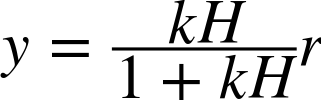
Now consider the steady state that prevails when all transients have died away. The input r is a constant, and (in the steady state) so is the output of the plant H itself. But under those circumstances, the fraction in the equation just displayed is always less than 1,^[23] so that the output from the feedback loop y will always be smaller than the reference value r! As the controller gain k is increased, the fraction will approach 1 and so the steady-state error is reduced. But no finite controller gain will succeed in eliminating it.

A Worked Example

Near the end of Chapter 3, we simulated a simple system that reproduced its input but delayed by a single time step. With proportional control, the system could be made to converge to a steady state under certain conditions but always exhibited a noticeable deviation from the setpoint value. We can now calculate the final value that the system converged to.

The system or “plant” H in the example neither increases nor decreases the value of its input; it merely delays it. So as far as the magnitude of the output is concerned, H has no influence and we can replace it with a multiplication by 1. However, the controller K changes the magnitude of its input by a factor of the “controller gain” k. If we again consider only the change in the magnitude, then the feedback formula becomes

For the graphs in Figure 3-4, we used values for the controller gain of k = 0.8 and k = 1.1 while keeping the setpoint constant at r = 1. The feedback formula now tells us that the magnitude of the steady-state output should be and , respectively; these values are also indicated in the figures. (For the unstable case of k = 1.1, this result is misleading, of course, because in this scenario the system never settles down to a steady state.)