By construction, the transfer functions for feedback systems tend to be proper rational functions—that is fractions of one polynomial in s over another polynomial in s:

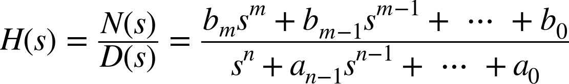
This fact is a consequence of the way transfer functions arise as solutions of linear differential equations with constant coefficients via Laplace transforms. (If the dynamics include time delays, then additional factors of the form e^–sT occur in the transfer function—more on this issue later in this chapter.)

The degree of a polynomial is the power of its highest term. In the preceding formula, the numerator is of degree m, and the denominator is of degree n. A transfer function is called strictly proper if it tends to 0 for large s, and it is called proper if it tends to a finite value as s approaches infinity. For transfer functions that are strictly rational functions, this means that for a transfer function to be strictly proper, the degree of the numerator polynomial must be less than the degree of the denominator polynomial (m < n) and that the degrees must be equal (m = n) for a transfer function to be proper. The rank R of a transfer function is the excess of numerator zeros over denominator zeros: R = m − n. Transfer functions of physical systems are never improper.

It is always possible to factor a polynomial (in the complex plane). If we factor both the numerator and the denominator polynomials of H(s), we obtain the standard or “root locus” form of the transfer function:

If s equals any of the z_k (for k = 1, ..., m) then the transfer function vanishes; hence the z_k are the locations of the zeros of H(s), or simply its zeros. Similarly, whenever s becomes equal to any of the p_k(for k = 1, ..., n – r), the denominator of H(s) vanishes and so the transfer function H(s) “blows up” for that value of s. Such positions are called the poles of H(s). Finally, if r > 0 then H(s) has a pole of order r at the origin; in that case, one says that H(s) is of type r.

Knowing only the poles and zeros of a transfer function allows us to understand a good deal about the dynamic response of the corresponding system. To see why, we need to understand what poles and zeros can tell us about dynamic behavior.

The effect that zeros have is easy to see: because y(s) = H(s)u(s), the output y(s) is zero whenever H(s) is zero irrespective of the input u(s). Moreover, for values of s near a zero, even though H(s) will not vanish exactly, it will still be small, so that the y(s) will also be small in a neighborhood of a transfer function zero. Zeros block the transmission of signals.

To understand the effect that poles have, we need to work a little harder. We begin with the transfer function in its standard, factored form. Such a rational function can always be split into partial fractions. In other words, we can find coefficients A_k such that

To understand how the system responds to a disturbance, we must transform the transfer function back into the time domain. This is now easy to do because we can perform the inverse transformation term by term. According to Table 20-1, an expression of the form 1/(s – p) in the frequency domain leads to e^pt in the time domain. Each pole p_k contributes an exponential term of the form e^p_kt to the transfer function in the time domain. The transfer function in the time domain is therefore a linear combination of exponentials, one for each pole:

Because the transfer function is a representation of the dynamic response of the system, it follows that the dynamic behavior can be expressed as a superposition of “modes.” The behavior of each mode is given by the exponential e^p_kt, where p_k is the position of the corresponding pole.

The dynamic behavior of each mode in the time domain now depends on the value of p_k. If p_k is real and negative, then the dynamic response e^p_kt will decay exponentially; the more negative p_k is, the faster is the decay. If p_k is real and positive, then the mode will grow exponentially with time.

But p_k does not need to be real; it can have an imaginary part. In this case, the dynamic response is oscillatory. Recall that the exponential function with a purely imaginary argument can be expressed in terms of trigonometric functions (also see Appendix C):

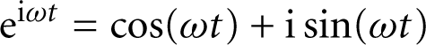
The greater ω is, the faster the wiggles.

If the pole is purely imaginary (p_k = iω_k), then the dynamic response consists of an oscillation with a constant amplitude. If the pole is complex—that is, if it has both a real and an imaginary part (p_k = σ_k + iω_k)—then the amplitude of the oscillation will either grow or decay exponentially, depending on the sign of the real part σ_k:

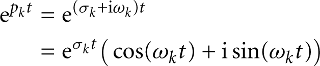
The first term describes the development of the amplitude, and the second term simply wiggles with frequency ω_k. The combination describes an oscillation with time-varying amplitude.

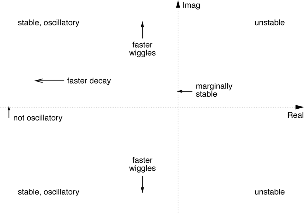
To summarize: the dynamic response is a linear combination of modes, one for each pole. The position of the pole determines the nature of the mode. The most important distinction concerns the sign of the real part of the pole. If the real part is positive, the amplitude of the corresponding mode will grow in time: the system blows up; it is unstable. Only poles with a negative real part describe stable behavior. In other words, for a system to be stable, all of its poles must be in the left-hand plane. Furthermore, poles with an imaginary part are associated with an oscillatory dynamic response; and the greater (in absolute terms) the imaginary part, the faster the oscillation. (See Figure 23-1.)

Special Cases and Additional Details

The preceding discussion skipped a few details and special cases, which we still need to mention.

Complex conjugate poles

If you consider the time response of a pole with an imaginary part, it may appear as if there will be an imaginary time response. After all, if p_k = σ_k + iω_k then the corresponding mode e^σ_kt(cos(ω_kt) + i sin(ω_kt)) seems to include an imaginary part (namely, the sine term). But this is not, in fact, the case. By construction, complex poles in the transfer function for a physical system always occur in complex conjugate pairs, so that if p_k = σ_k + iω_k is a pole, then there will also be a pole p_k+1 = σ_k – iω_k. Moreover, the corresponding coefficients A_k and A_k+1 in the partial fraction expansion will also be complex conjugates of each other. Both p_k and p_k+1 lead to oscillatory modes with the same frequency, but their respective imaginary parts cancel each other out! The end result is that a complex pole, together with its complex conjugate, contributes a purely real oscillatory mode to the dynamic response in the time domain.

Figure 23-1. Pole positions in the complex plane and how they determine the nature of the dynamic behavior in the time domain.

Multiple poles

It may be that the partial fraction expansion of the transfer function contains terms with the denominator raised to some power:

In this case, the corresponding pole is called a multiple pole of order μ. According to Table 20-1, the time response for such a term picks up an additional factor of t^{μ – 1}:

Finally, if a term A_j/(s – p_j)^μ occurs in the partial fraction expansion, then all terms of lower power (A_k/(s – p_j), A_ℓ/(s – p_j)², ..., A_m/(s – p_j)^μ–1) will also occur.

Poles on the imaginary axis

If a pole is purely imaginary (that is, if its real part is zero) then the pole is located on the imaginary axis. The amplitude of the corresponding mode neither increases nor decreases with time, and the mode is said to be marginally stable. This is not the case if the pole in question is a multiple pole, because the additional factors of t in the time response for multiple poles make multiple poles on the imaginary axis unstable.

Pole/zero cancellations

It is possible for a pole and a zero to occur at the same location: p_k = z_j. In that case, the respective factors in the transfer function will cancel. This effect is sometimes introduced intentionally to suppress an undesired mode, as when additional elements are added to the control loop in order to create a zero at or near the pole of the undesired mode. Even if the cancellation is not perfect, the effect of this operation will be a much reduced amplitude of the mode in question.

Figures showing the positions of poles and zeros in the complex plane are known as pole-zero diagrams. Poles are indicated using × symbols, and zeros are indicated with open circles. The nature of the system’s dynamic behavior can be read off from a pole-zero diagram; Figure 23-3 shows a selection of pole configurations in the complex plane together with the associated dynamic response to a short impulse at . The basic rules are as follows:

Dominant Poles

If we are dealing with a transfer function of high order (many poles and zeros), then we can often simplify the analysis by concentrating only on the dominant poles and neglecting the other ones. Poles that can be neglected are those that are far to the left of the dominant poles: the dynamic response of the neglected poles will decay quickly, so they will not exert a major influence on system behavior. We can also neglect poles that are close to a zero; the amplitude of the associated mode will be very small and, again, ignoring such a pole won’t change the observed behavior much. (See Figure 23-2.)

Figure 23-2. Dominant poles in red and subdominant poles in green. In the right-hand graph, the pole on the real axis is subdominant because it is nearly canceled by the nearby zero.

Figure 23-3. Pole configurations and their corresponding impulse responses. In panel B, the green curve decays as fast as the red curve but wiggles faster (vertical pole movement), whereas the blue curve oscillates at the same frequency as the red one but decays faster (horizontal pole movement). In panel C, the blue pole at the origin is a double pole (indicated by the “2”), and its dynamic response grows linearly with time. In panel D, the curves correspond to the blue pair of poles and either the red or the green pole. The green pole is far from the origin and hardly affects the dynamic response, but the red pole is close to the origin and therefore determines the dominant, slow decay of the red curve.

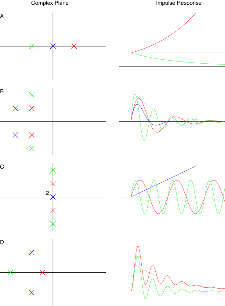
The time response in panel D of Figure 23-3 consists of the contribution of the blue poles and either the red or the green pole. The blue pair of complex conjugate poles describes a damped oscillation. The green pole, which is farther away from the origin than the blue poles, describes a mode that decays so quickly that it hardly affects the dynamic response at all. The red pole, however, is closer to the origin than the blue poles. Its corresponding mode in the time domain decays more slowly than the oscillations due to the complex conjugate pair. The red pole is a typical dominant or “slow” pole.

Pole Placement

Knowing how the dynamic response of a system is determined by the position of the system’s poles, we can attempt to design a system with the desired behavior by “moving its poles”—a process known as pole placement. Controller tuning (see Chapter 9) is a simple example of pole placement: we try to adjust the controller gains in order to “move the poles” into positions corresponding to the desired performance. The root locus method (Chapter 24) is a graphical design technique based on the idea of moving poles in the complex plane.

At the beginning of Chapter 9 we listed several goals for the tuning process, such as the typical response time of the system, the amount of overshoot after a disturbance, the damping of oscillations, and so on. These quantities can be related directly to pole positions.^[24] Specifying numerical values for the tuning goals therefore amounts to restricting the system’s poles to a specific region of the complex plane. Controller tuning can now be regarded as a process of moving the dominant poles into the permissible regions.

But we are not limited to adjusting the controller gains. One can insert additional elements with known transfer functions into the control loop, a process known as “loop shaping.” For instance, one can introduce a “lead/lag compensator” with transfer function

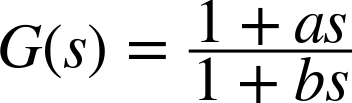
into the control loop. This compensator has a pole at –1/b and a zero at –1/a. We can now adjust a such that the zero coincides (for example) with an undesirable pole and fix b to place the corresponding pole into favorable position.

All the preceding considerations assume that the transfer function is, in fact, a purely rational function: one polynomial in s divided by another polynomial in s. If the dynamics of the system can be expressed entirely in terms of a linear differential equation with constant coefficients, then this assumption will be satisfied. But it will not be satisfied if the system dynamics include pure time delays.

In physical systems, delays often arise because energy or material is transported over some distance: if water needs to flow through a hose or pipe, then there will be a delay from the time the faucet was opened to the time the water level in the bucket begins to rise. Symbolically, the output of a system H is delayed by some time τ relative to the input

Time delays are not described by linear differential equations with constant coefficients, and their transfer functions are not purely rational functions—instead, time delays introduce exponential factors of the form e^–sτ into the transfer function. This is less of a mathematical problem (the transfer functions remain well behaved) but it is a major practical inconvenience. Many analytical methods in control theory rely on the transfer function being the ratio of two polynomials. (For instance, the ability to perform a partial fraction expansion—which was central to our description of the dynamic response in terms of modes and their associated poles—requires the transfer function to be a rational function.)

In order to retain the desired structure of the transfer function, one approximates the exponential factor e^–sτ either by a power series or by a rational function approximation. All of these approximations are good as long as sτ is small—that is, for time scales that are long compared to the duration of the delay.

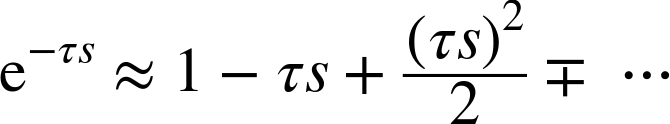
The Taylor expansion of the exponential function is familiar, but it is not a good approximation unless sτ is quite small:

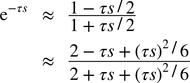
Much better results can be obtained by approximating the exponential function through a rational function instead of a power series (Padé approximation). The following two approximations are often used:

Finally, we can make use of the identity , and thereby arrive at an approximation for the exponential function, by plugging in some “large,” but finite value of n (say, n = 5, ..., 20):

This approximation has a nice interpretation as a sequence of n lags, each with time constant τ/n. The value of n should not be too large, because otherwise the expression becomes numerically unstable.

Finally, keep in mind that all of these formulas are only approximations. Not only do they have a limited range of validity, but using them does also change the pole structure of the transfer function. The results should therefore be used with care!