
Chapter 10. Implementation Issues
Implementing a feedback loop based on a PID controller involves some low-level choices in addition to the overall concerns about stability and performance.
Actuator Saturation and Integrator Windup
In principle, there is no limit on the magnitude of the controller’s output: when the controller gain is sufficiently large, the controller output u can become arbitrarily large. But it’s a whole different question whether the downstream system (the “plant”) will be able to follow this signal. It may either not have enough “power” to respond to an arbitrarily large input, or we may run into an even more fundamental limitation.
Think of a heated room. Given a high enough setting on the dial, the desired heat output from the central heating system can be very large—quite possibly larger than the amount of heat the heating system can actually produce. But even more dramatic is the opposite scenario in which we select a desired temperature that is lower than the current room temperature. In this case, the best the controller can do is to switch the heat off—there is no way for it to actively lower the temperature in the room (unless it is coupled to an air conditioning unit).
Such limitations always exist. In the case of a pool of compute servers, the maximum number of servers is limited: once they are all online, further demands from the controller will have no effect. At the other extreme, the number of active servers can never fall below zero. And so on.
In classical control engineering, the system that translates the controller output to an actual physical action is called the actuator (such as the motor that drives a valve). When an actuator is fully engaged (that is, either fully open or completely closed), it is said to be saturated. Hence the problem of a controlled system being unable to follow the controller output is known as actuator saturation.
Actuator saturation is something to be aware of. It places fundamental limitations on the performance of the entire control system. These limitations will not show up in an analysis of the transfer function: the transfer function assumes that all components are linear, and saturation effects are profoundly nonlinear. Instead, one must estimate the magnitude of the largest expected control signals separately and evaluate whether the actuator will be capable of following them. In simulations, too, one must be sure to model accurately the system’s real-world limitations.
During production, the control system should rarely reach a saturated state (and it is probably a good idea to trigger an alert when it does). However, it is not safe to assume that “it won’t happen”—because it will, and more often than one might suppose.
Preventing Integrator Windup
Actuator saturation can have a peculiar effect when it occurs in a control loop involving an integral controller. When the actuator saturates, an increased control signal no longer results in a correspondingly larger corrective action. Because the actuator is unable to pass the appropriate values to the plant, tracking errors will not be corrected and will therefore persist. The integrator will add them up and may reach a very large value. This will pose a problem when the plant has “caught up” with its input and the error changes sign: it will now take a long time before the integrator has “unwound” itself and can begin tracking the error again.
To prevent this kind of effect, we simply need to stop adding to the integral term when the actuator saturates. (This is known as “conditional integration” or “integrator clamping.”) Like the actuator saturation that causes it, integrator windup should not happen during production, but it occurs often enough that mechanisms (such as clamping) must be in place to prevent its effects.
Setpoint Changes and Integrator Preloading
The opposite problem occurs when we first switch the system on or when we make large setpoint changes. Such sudden changes can easily overload (saturate) the actuators. In such cases, we may want to preload the integral term in the controller with an appropriate value so that the system can respond smoothly to the setpoint change. (This is known as bumpless transfer in control theory lingo.)
As an example, consider the server pool described in Chapter 5. The entire system is initially offline, and we are about to bring it up. We may know that we will need approximately 10 active server instances. (Ultimately, we may need 8 or we may need 12, but we know it’s in that vicinity.) We also know the value of the coefficient ki of the integral term in the controller. In the steady state, the tracking error e will be zero and so the contribution from the proportional term kp e will vanish. Therefore, the entire control output u will be due to the integral term ki I. Since we know that u should be approximately 10, it follows that we should preload the integral term I to 10/ki.
Smoothing the Derivative Term
Whereas the integral term has a tendency to smooth out noise, the derivative term has a tendency to amplify it. That’s inevitable: the derivative term responds to change in its input and noise consists of nothing but rapid change. However, we don’t want to base control actions on random noise but on the overall trend in the tracking error. So if we want to make use of the derivative term in a noisy system, we must get rid of the noise—in other words, we need to smooth or filter it.
Most often, we will calculate the derivative by a finite-difference approximation. In this approximation, the value of the derivative at time step t is

where et is the tracking error at time step t and δt is the length of the time interval between successive steps.
In a discrete-time implementation, recursive filters are a convenient way to achieve a smoothing effect. If we apply a first-order recursive filter (equivalent to “exponential smoothing”) to the derivative term, the result is the following formula for the smoothed discrete-time approximation to the derivative ![]() at time step t:
at time step t:

The parameter α controls the amount of smoothing: the smaller α is, the more strongly is high-frequency noise suppressed.
The parameter α introduces a further degree of freedom into the controller (in addition to the controller gains kp, ki, and kd), which needs to be configured to obtain optimal performance. This is not easy: stronger smoothing will allow a greater derivative gain kd but will also introduce a greater lag (in effect, slowing the controller input down), thus counteracting the usual reason that made us consider derivative action in the first place. Nevertheless, a smoothed derivative term can improve performance even in noisy situations (see Chapter 16 for an example).
Finally, it makes no difference whether we smooth the error signal before calculating the derivative (in its discrete-time approximation) or instead apply the filter to the result (as was done in the preceding formula). When using a filter like the one employed here, the results are identical (as a little algebra will show).
Choosing a Sampling Interval
How often should control actions be calculated and applied? In an analog control system, whether built from pipes and valves or using electronic circuitry, control is applied continuously: the control system operates in real time, just as the plant does. But when using a digital controller, a choice needs to be made regarding the duration of the sampling interval (the length of time between successive control actions).
When controlling fast-moving processes in the physical world, computational speed may be a limiting factor, but most enterprise systems evolve slowly enough (on a scale of minutes or longer) that computational power is not a constraint. In many cases we find that the process itself imposes a limit on the update frequency, as when a downstream supplier or vendor accepts new prices or orders only once a day.
If we are free to determine the length of the sampling interval, then there are two guiding principles:
- Faster is better...
In general, it is better to make many small control actions quickly than to make few, large ones. In particular, it is beneficial to respond to any deviation from the desired behavior before it has a chance to become large. Doing so not only makes it easier to keep a process under control, but it also prevents large deviations from affecting downstream operations.
- ... unless it’s redundant.
On the other hand, there is not much benefit in manipulating a process much faster than the process can respond.
An additional problem can occur when using derivative control. If the derivative is calculated by finite differencing, then a very short interval will lead to round-off errors, whereas an interval that is too long will result in finite-differencing errors.
Ultimately, the sampling interval should be shorter (by a factor of at least 5 to 10) than the fastest process we want to control. If the controlled process or the environment to which the process must respond changes on the time scale of minutes, then we should be prepared to apply control actions every few seconds; if the process changes only once or twice a day, then applying a control action every few minutes will be sufficient.
(A separate concern is that the continuous-time theory, as sketched in Part IV, is valid without modifications only if the sampling interval is significantly shorter than the plant’s time constant. If this condition is not fulfilled, then the discreteness of the time evolution must be taken into account explicitly in the theoretical treatment. See Chapter 26.)
Variants of the PID Controller
In Chapter 4 we saw that a PID controller consists of three terms, which in the time domain can be written as follows:
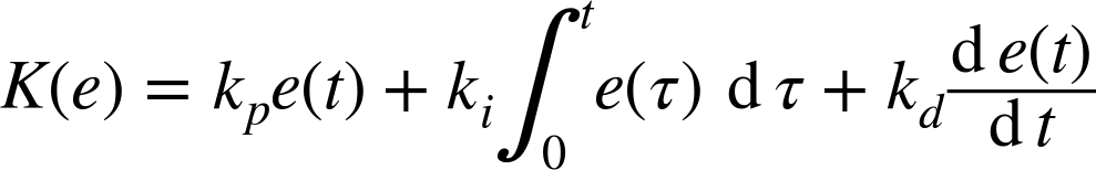
Here e(t) is the tracking error, e(t) = r(t) – y(t). A couple of variants of this basic idea exist, which can be useful in certain situations.
Incremental Form
It is sometimes useful simply to calculate the change in the control signal and send it to the controlled system as an incremental update. In the control theory literature, this is called the “velocity form” or “velocity algorithm” of the PID controller.
For a digital PID controller, the incremental (or velocity) form is straightforward. We find that the update at time step t in the control signal Δut is

When the derivative term is missing (kd = 0), the equation for the incremental PID controller takes on an especially simple form.
The incremental form of the controller is the natural choice when the controlled system itself responds to changes in its control input. For instance, we can imagine a data center management tool that responds to commands such as “Spin up five more servers” or “Shut down seven servers” instead of maintaining a specific number of servers.
In a similar spirit, during the analysis phase it is sometimes more natural to think about the changes that should be made to the system in response to an error rather than about its state. But if the plant expects the actual desired state as its input (such as: “Maintain 35 server instances online”), then it will be necessary to insert an aggregator (or integrator) between the incremental controller and the controlled plant. This component will add up all the various control changes Δu to arrive at (and maintain) the currently desired control input u. (Combining the aggregator with the incremental controller leads us back to the standard PID controller that we started with.)
Finally, because the incremental controller does not maintain an integral term, no special provisions are required to avoid actuator saturation or to achieve bumpless transfers. Both of these phenomena arise from a lack of synchronization between the actual state of the controlled system and the internal state of the controller (as maintained by the integral term). Since an incremental controller does not maintain an internal state itself, there is only a single source of memory in the system (namely, in the aggregator or plant); this naturally precludes any possibilities of disagreement. (The control strategy described in Chapter 18 shows this quite clearly. In this case, the aggregator takes the saturation constraints of the controlled system into account when updating its internal state—without the controller needing to know about it.)
Error Feedback Versus Output Feedback
In general, the controller takes the tracking error as input. There is an alternative form, however, that (partially) ignores the setpoint and bases the calculation of the control signal only on the plant output. Its main purpose is to isolate the plant from sudden setpoint changes.
To motivate this surprising idea, consider a PID controller that includes a derivative term to control a system, operating in steady state, at a setpoint that is held constant. Now suppose we suddenly change the setpoint to a different value. If the controller is working on the tracking error r(t) – y(t), then this change has a drastic effect on the derivative terms: although the plant output y(t) may not change much from one moment to the next, the setpoint r(t) was changed in a discontinuous fashion. Since the derivative of a discontinuous step is an impulse of infinite magnitude, it follows that the sudden setpoint change will lead to a huge signal being sent to the plant, its magnitude limited only by the actuator’s operating range. This undesirable effect is known as the “derivative kick” or “setpoint kick.”
Now consider the same controller but operating only on the (negative) plant output –y(t). Since the setpoint r(t) was held constant (except for the moment of the setpoint change), the effect of the derivative controller operating only on y(t) is exactly the same as when it was operating on the tracking error r(t) – y(t), but without the “derivative kick.”
To summarize: if the setpoint is held constant except for occasional steplike changes,
then the derivative of the output ![]() is equal to the derivative of the tracking error
is equal to the derivative of the tracking error ![]() except for the infinite impulses that occur when the setpoint
r(t) undergoes a step change. So in this
situation, basing the derivative action of a PID controller on only the output
y(t) has the same effect as taking the
derivative of the entire tracking error r(t) –
y(t). Furthermore, taking the derivative of the
output only also avoids the infinite impulse that results from the setpoint changes.
except for the infinite impulses that occur when the setpoint
r(t) undergoes a step change. So in this
situation, basing the derivative action of a PID controller on only the output
y(t) has the same effect as taking the
derivative of the entire tracking error r(t) –
y(t). Furthermore, taking the derivative of the
output only also avoids the infinite impulse that results from the setpoint changes.
Similar logic can be applied to the proportional term. Only the integral term must work on the true tracking error. The most general form of this idea is to assign an arbitrary weight to the setpoint in both the proportional and derivative terms. With this modification, the full form of the PID controller becomes

with 0 ≤ a, b ≤ 1. The parameters a and b can be chosen to achieve the desired response to setpoint changes. The entire process is known as “setpoint weighting.”
The General Linear Digital Controller
If we use the finite-difference approximations to the integral and the derivative, then the output ut at time t of a PID controller in discrete time can be written as

where et = rt – yt. If we plug the definition of et into the expression for ut and then rearrange terms, we find that ut is a linear combination of rθ and uθ for all possible times θ = 0, ..., t.
In the case of setpoint weighting, we allowed ourselves greater freedom by introducing additional coefficients (et = a rt – yt in the proportional term and et = b rt – yt in the derivative term). Nothing in ut changes structurally, but some of the coefficients are different. (Setting a = b = 1 brings us back to the standard PID controller.)
Generalizing even further, we have the following formula for the most general, linear controller in discrete time:
All controllers that we have discussed so far—including the standard PID version, its setpoint-weighted form, the incremental controller, and the derivative-filtered one—are merely special cases obtained by particular choices of the coefficients a0, ..., at and b0, ..., bt. Further variants can be obtained by choosing different coefficients.
Nonlinear Controllers
All controllers that we have considered so far were linear, which means that their output was a linear transformation of their input. Linear controllers follow a simple theory and reliably exhibit predictable behavior (doubling the input will double the output). Nevertheless, there are situations where a nonlinear controller design is advisable or even necessary.
Error-Square and Gap Controllers
Occasionally the need arises for a controller that is more “forgiving” of small errors than the standard PID controller but at the same time more “aggressive” if the error becomes large. For example, we may want to control the fill level in an intermediate buffer. In such a case, we neither need nor want to maintain the fill level accurately at some specific value. Instead, it is quite acceptable if the level fluctuates to some degree—after all, the purpose of having a buffer in the first place is for it to neutralize small fluctuations in flow. However, if the fluctuations become too large—threatening either to overflow the buffer or to let it run empty—then we require drastic action to prevent either of these outcomes from occurring.
A possible modification of the standard PID controller is to multiply the output of the controller (or possibly just its proportional term) by the absolute value of the tracking error; this will have the effect of enhancing control actions for large errors and suppressing them for small errors. In other words, we modify the controller response to be

Because it now contains terms such as |e|e, this form of the controller is known as an error-square controller (in contrast to the linear error dependence of the standard PID controller). This is a rather ad hoc modification; its primary benefit is how easily it can be added to an existing PID controller.
Another approach to the same problem is to introduce a dead zone or “gap” into the controller output. Only if (the absolute value of) the error exceeds this gap is the control signal different from zero.
Both the error-square form of the controller and introduction of a dead zone are rather ad hoc modifications. The resulting controllers are nonlinear, so the linear theory based on transfer functions applies “by analogy” only.
Simulating Floating-Point Output
By construction, the PID controller produces a floating-point number as output. It is therefore suitable for controlling plants whose input can also take on any floating-point value. However, we will often be dealing with plants or processes that permit only a set of discrete input values. In a server farm, for instance, we must specify the number of server instances in whole integers.
The naive approach, of course, is simply to round (or just truncate) the floating-point output to the nearest integer. This method will work in general, but it might not yield very good performance owing to the error introduced by rounding (or truncating). A particular problem are situations that require a fractional control input in the steady state. For instance, we may find that precisely 6.4 server instances are required to handle the load: 6 are not enough, but if we deploy 7 then they won’t be fully utilized. Using the simple rounding or truncating strategy in this case will lead to permanent and frequent switching between 6 and 7 instances; if random disturbances are present in the loop, then the switching will be driven primarily by random noise. (We will encounter this problem in the case studies in Chapter 15 and Chapter 16.)
Given the integer constraints of the system, it won’t be possible to generate true fractional control signals. However, one can design a controller that gives the correct output signals “on average” by letting the controller switch between the two adjacent values in a controlled manner. Thus, to achieve an output of 6.4 “on average,” the controller output must equal 6 for 60 percent of the time and 7 for 40 percent of the time. For this strategy to make sense, the controller output must remain relatively stable over somewhat extended periods of time. If that condition is fulfilled, then such a “split-time” controller can help to reduce the amount of random control actions.
Categorical Output
Permissible control inputs can be even more constrained than being limited to whole integers. For instance, it is conceivable that the allowed values for the process input are restricted to nonnumeric “levels” designated only by such categorical labels as “low,” “medium,” “high,” and “very high.”
These labels convey an ordering but no quantitative information. Hence the controller does not have enough information about the process (and its levels) to select a particular level. The only decision the controller can make is whether the current level should be incremented (or decremented) in response to the current sign and magnitude of the error.
Because it has only a few, discrete control inputs, such a system will usually not be able to track a setpoint very accurately; however, it may still be possible to restrict the process output to some predefined range of values. We will study an example of such a system in Chapter 18.