
Chapter 5
The U.S. Mortgage Market
Mortgage Market Snapshot
History: After the Great Depression, the United States federal government created several government and government-sponsored agencies in order to provide government-guaranteed mortgage insurance and create a liquid secondary market so that more loans could be issued. The secondary mortgage market in the United States became active in the 1970s, and extended to the private sector when Bank of America National Trust & Savings Association became the first truly private issuer of mortgage-backed securities in 1977. The secondary mortgage market reached great heights by the mid-2000s; however, with the recent subprime mortgage crisis, people have been rethinking the ways in which mortgage-related instruments have been packaged and issued.
Size: Total outstanding mortgage-related debt in the United States is about $14.1 trillion as of the first quarter of 2010, according to the Federal Reserve.
Products: Today's market offers investors an array of investment options, ranging from simple generic pass-through bonds to a diverse set of structured mortgage-backed securities (MBSs) with very complicated cash flow patterns.
First Usage: In 1970, the Government National Mortgage Association, or Ginnie Mae, issued the first mortgage pass-through security that passed the principal and interest payments on mortgages to investors by pooling together qualified mortgage loans.
Selection of Famous Events:
1994: Harris Trust and Savings Bank, a subsidiary of the Bank of Montreal, suffered losses of $51.3 million from investments in risky mortgage derivatives that were supposedly kept in low-risk institutional customer accounts.
2007: In August 2007, rising defaults in subprime loans rattled not only the secondary mortgage market, but also financial markets in general. Many feared that Countrywide Financial, the largest mortgage lender in the United States, would teeter toward bankruptcy. Indeed, first, it accepted a credit line of $11.5 billion from banks, then later a financing of $2 billion from Bank of America, which eventually acquired the mortgage lender in 2008 for about $4 billion in stock. Countrywide announced a $1.2 billion third-quarter loss in October 2007, its first reported loss in 25 years. In addition to tremendous losses on subprime loans, the mortgage lender was also under FBI investigation for mortgage fraud, including misleading investors about the extent of the credit risk involved in maintaining its market operations.
2007–2008: Lehman Brothers Holdings Inc. was a global financial services firm that was also hit hard by the subprime mortgage crisis. By 2007, the firm closed down its subprime lender, BNC Mortgage, took an after-tax charge of $25 million, and a goodwill write down of $27 million due to poor market conditions in the mortgage realm. However, Lehman continued to suffer from the continuing subprime mortgage crisis. With falling stock share prices and rising losses in low-rated mortgage securities, it eventually succumbed to bankruptcy in 2008, while posting a third-quarter loss of $3.9 billion. Lehman's bankruptcy filing sparked worries around the world about the health of the global financial system.
Applications: Mortgage-backed securities can be used to satisfy specific risk preferences on a number of dimensions, including prepayment, duration, and credit risk.
Users: Investors in the secondary mortgage market include investment banks as well as corporations and individual investors.
INTRODUCTION
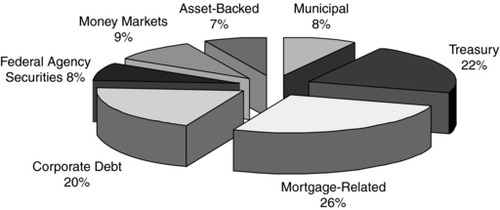
In 1970, when the Government National Mortgage Association (Ginnie Mae) issued its first mortgage pass-through security, the secondary mortgage market was little more than an inchoate assemblage of government housing initiatives. Today, total outstanding mortgage-related debt is over $10 trillion, making mortgages the largest segment of the U.S. bond market (see Exhibit 5.1). The structure of the market has also undergone a significant change.
Exhibit 5.1 Outstanding U.S. Bond Market Debt, Q4 2009
Source: Securities Industry Financial Markets Association (SIFMA).
The growth in market size was accompanied by a broad-based expansion in the variety of mortgage-derivative products available to investors. Today's market offers investors an array of investment options ranging from simple generic pass-through bonds, like those first issued by Ginnie Mae in 1970, to a diverse set of structured products with very complicated cash-flow patterns, designed to satisfy specific risk preferences on a number of dimensions including prepayment, duration, and credit risk. Many of the changes in the market for mortgage-backed securities since the early 1970s can be attributed to the theoretical, methodological, and computational achievements of financial engineering during the same time period. The story of the evolution of the market for mortgage-backed securities is entwined with the evolution of financial engineering as a discipline.
The one factor that distinguishes MBSs from most other fixed-income products is the uncertainty of the cash flows and the consequential complexity of the valuation process. The primary reason for the uncertainty is that borrowers hold an option to prepay their mortgages. If, and when, a borrower exercises this option depends on general economic conditions (e.g., interest rates, home price appreciation) and circumstances specific to each borrower (e.g., relocation, divorce, job loss). An estimate of the cash flow at a future point in time requires an estimate of the probability that a loan will prepay at that point. The expected future probability that a borrower will exercise the prepayment option may be characterized as being dynamic, path dependent, and uncertain. It is dynamic in the sense that it changes over time; path dependent in the sense that at any point in time it depends on current and previous states of the world; and uncertain in the sense that at the time of valuation it requires knowledge of future states of the world.
Thirty-five years ago, the tools, methods, and computing power required to properly value mortgage-backed securities were not generally available to investors. The prevailing method of valuation was cash flow yield (also known as mortgage yield). This is a static method that does not properly capture the value of the prepayment option. Out of necessity, the decision to invest in an MBS was made with very little information about the underlying collateral, and very little understanding of how the characteristics of the borrowers might impact cash flows.
Today's investors, in contrast, have access to tools that allow them to routinely process and analyze massive amounts of loan-level information in short periods of time and use this information to value very complex mortgage derivatives. This capability is largely due to advances in financial engineering, which has championed the development of high-speed, theoretically sound valuation methods that employ simulation techniques to value the prepayment option. The development of sophisticated valuation tools has, in turn, led to the development of a more diverse set of mortgage-derivative products that better meet the preferences of investors.
This chapter is a discussion of the evolution of the market for mortgage-backed securities (or the secondary mortgage market), its institutions, participants, products, and analytic methods, and the role of financial engineering. We begin with a discussion of government housing policy and its role in the establishment of the market. This is a brief but important discussion, insofar as understanding the current state of the MBS market and its future direction is concerned. Indeed, the housing policy established by Congress 50 or even 80 years ago lies at the heart of our current economic situation, and will for the foreseeable future. Having established the institutional framework of today's mortgage market, we proceed to discuss the historical development of the suite of mortgage derivatives currently available to investors. As we will see, the evolution of the different types of mortgage-backed securities available to investors reflects the development of financial engineering methods. We then discuss the current state of mortgage valuation with an emphasis on the role of prepayments and defaults. The information available to value a MBS, and the computational ability to process that information, have changed significantly over the history of the secondary mortgage market. In fact, this is an area that has seen major advances in the past 8 to 10 years. In the final section, we discuss current market conditions, the future of key institutions, and the role of financial engineering in the mortgage market of the future.
A BRIEF HISTORY OF THE ORIGIN OF THE MARKET FOR MORTGAGE-BACKED SECURITIES
The secondary market for mortgages, and the history of mortgage-backed securities in general, has its roots in the Great Depression. In 1934, Congress passed the National Housing Act, which established the Federal Housing Authority (FHA). The legislation was enacted in response to the very high rate of mortgage defaults between 1929 and 1934. By some estimates, homeowner default rates were as high as 25 to 30 percent nationally. The defaults were driven by a combination of high unemployment, a steep decline in housing prices, and the practice of issuing balloon mortgages.1
The FHA was established to provide insurance on mortgages issued by FHA-approved lenders. The intent of the program was to encourage lending by reducing the risk of loss associated with a mortgage default. The mortgage insurance premium was paid by the borrower through an increase in monthly payments. The FHA insurance program is still in existence, and has played a very important role in the recent housing crisis. In addition to providing insurance to lenders, the underwriting standards on FHA-approved loans are less stringent than those of standard mortgages. Borrowers can secure an FHA loan with a very small cash investment, and income requirements are less rigorous than standard mortgages. The FHA is currently part of the Department of Housing and Urban Development (HUD).
In 1938, using authority granted under the National Housing Act of 1934, the FHA chartered the Federal National Mortgage Association (Fannie Mae). The purpose of establishing Fannie Mae was to provide liquidity to the mortgage market by creating a secondary market for mortgages. Fannie Mae bought FHA-insured mortgages from lenders and either held them in its own portfolio or sold them to investors. Lenders were motivated to underwrite FHA-insured loans, since they were confident that they could sell them. Selling the loans provided lenders with new capital to write additional loans. Creating a secondary market for mortgages also facilitated the flow of capital across geographic regions, which is critical for a market such as housing that is inherently local. In the late 1940s Fannie Mae expanded its buying program to include loans guaranteed by the Veterans Administration (VA).
In 1968, the Federal National Mortgage Association was split into two entities, one public and one privately owned. The privately owned entity kept the name Fannie Mae, and the publicly owned entity was named the Government National Mortgage Association (Ginnie Mae). The establishment of these two entities was an important step by the federal government toward expanding the secondary market for mortgages, and advancing its policy of providing housing assistance to Americans. Ginnie Mae was specifically created to expand affordable housing. In 1970, the government established a third entity, the Federal Home Loan Mortgage Corporation (Freddie Mac), which, like Fannie Mae, was privately owned. One of the primary reasons for establishing Freddie Mac was so that Fannie Mae would not be a monopoly. These two institutions, Fannie and Freddie, are, technically, government-sponsored enterprises (GSEs), which means they are federally chartered, but privately owned. These two GSEs, plus Ginnie Mae, are collectively referred to as agencies. As a group, the agencies have been crucial to the development and robust growth of the secondary market for mortgages.
AGENCY MORTGAGE PASS-THROUGH SECURITIES
In 1970, Ginnie Mae introduced the first mortgage pass-through security, which effectively marked the beginning of the modern-day market for mortgage-backed securities. A mortgage pass-through is a bundle or pool of mortgages that have similar characteristics such as maturity, origination date, interest rate, mortgage type (fixed rate versus adjustable rate), and property type (single-family home or multifamily home). An investor who purchases a mortgage pass-through security is entitled to the principal and interest payments2 from the mortgages in the pool. Under the Ginnie Mae mortgage pass-through program, loans are pooled by approved issuers and resold in the secondary mortgage market. Ginnie Mae does not actually issue the securities, but it does guarantee the principal and interest payments of pools issued by its approved issuers.
Ginnie Mae took the lead in introducing mortgage pass-throughs, and the two GSEs eventually followed (Freddie Mac in 1972 and Fannie in 1981). It is important to note that unlike Ginnie Mae, the GSEs actually purchase mortgages, and then either retain them in their own portfolios or securitize and sell them in the secondary market. Also, in keeping with its mission of assisting low- and moderate-income home buyers, the Ginnie Mae pass-through program issues pools of mortgages that are primarily FHA insured or VA guaranteed. These loans are commonly referred to as government loans.
The vast majority of mortgage pass-through securities are traded in the to-be-announced (TBA) market. A TBA is a contract to buy or sell a set of pools or mortgages at some future date. The TBA market gets its name from the fact that the buyer does not know the specific pools that will be delivered until two days before delivery. The TBA market trades on the assumption that the pools are homogeneous and therefore fungible. As an example, an investor can enter into a contract to buy pass-throughs backed by Fannie Mae 5 percent, 30-year fixed-rate loans, but the investor will not know the average age of the loans in the pools, the average loan size, or even the average mortgage rate on the pools until 48 hours before delivery. TBAs settle according to a monthly schedule set by the Securities Industry Financial Markets Association (SIFMA). Mortgage originators use the TBA market to fund originations by negotiating contracts several months in advanced of the settlement date, effectively allowing them to lock in a price for mortgages that they are still in the process of originating. SIFMA also provides guidelines for “good delivery” of TBAs, which generally address settlement issues, such as the maximum number of pools that can be delivered per $1 million of TBAs, and the variance of the delivery amount of the trade and the agreed-upon amount.
Mortgage pass-throughs also trade as specified pools, meaning that investors can purchase pools for their specific characteristics, such as loan balance (low, medium, or high); geography (location of the homes underlying the pools); creditworthiness of the borrower; occupancy type (primary residence, investor owned); and property type (single-family residence, multifamily, condo, co-op). The specified pool market places special value on certain loan characteristics, and in that sense it is antithetical to the TBA market, which operates under the assumption of pool homogeneity. The specified pool market has become very active in the past five to six years, as the agencies have provided more information about the characteristics of the loans within the pools. For instance, in 2003 the agencies began reporting weighted averages and quartiles for FICO scores, loan-to-value (LTV) ratios, occupancy type, mortgage purpose (home purchase, cash-out refinance, rate refinance), and average loan size for all pools originating from 1996 onward. In early 2006, Freddie Mac began reporting loan-level information for the loans backing their pools, but, interestingly, it did not provide an indicator of which pool the loan belongs to, so the information is of limited use. However, the availability of this information, along with information on the geographic concentration of the loans within a pool, has spurred growth of the specified pool market. It has also provided investors with a wealth of information that they have used to improve MBS valuation models.
Agency Market Structure
MBS market segmentation is largely collateral-based in the sense that the segments reflect fundamental differences in borrower characteristics.3 Borrower characteristics are a key determinant of the expected probabilities of prepayment. Consequently, the market segmentation scheme reflects fundamental differences in security valuation. In effect, for a given state of the economy, each segment of borrowers has a different propensity to prepay. Market segments are important differences that must be accounted for in the valuation process. Advances in financial engineering since the creation of the MBS market have enabled investors to incorporate these differences into the valuation process.
Ginnie Mae pools are comprised of government-guaranteed loans primarily from the VA and FHA loan programs. GSE pools, unlike Ginnie Mae, do not limit securitization to pools backed by government-guaranteed loans. Most of the loans in GSE pools are nongovernment loans. These loans are referred to as conventional loans. Pools backed by conventional loans tend to have different prepayment speeds from pools backed by government loans. Part of the reason for this is that the government loan programs have higher loan-to-value (LTV) limits and the loans tend to be smaller.
Agency loan standards generally require that borrowers provide written proof (documentation) of employment and income. In addition, conventional loan standards typically require that borrowers have a loan-to-value ratio of less than 80 percent, satisfy a minimum level of creditworthiness, and meet certain minimum levels of debt-to-income ratios. Government loans often have LTVs higher than 80 percent. Nongovernment loans that do not meet GSE standards are typically securitized by private-label issuers and sold in the non-agency market.
All three agencies limit eligibility based on loan size, known as the conforming balance limit. In 2009 the conforming balance limit was $729,500 for temporary high-cost areas, $625,500 for permanent high-cost areas, and $417,000 in all other areas. The limit is reset annually based on the level of home price appreciation. Conventional loans that exceed the conforming balance limit are not eligible for securitization in an agency pool, and are referred to as jumbo loans. Securities backed by jumbo loans trade in the non-agency market.
One important feature of MBS market segmentation that is not based on borrower characteristics relates to credit risk. Setting aside differences in loan characteristics, from an investor's point of view Ginnie Mae pass-throughs and GSE pass-throughs are not perfect substitutes because of an important difference in the guarantee of principal and interest payments. All of the agencies guarantee investors the timely payment of principal and interest, but only the Ginnie Mae guarantee carries the full faith and credit of the U.S. government. The GSEs have traditionally been viewed as having the implicit guarantee of the U.S. government because of their GSE designation. In principle, because of the difference in the credit risk, GSE pass-throughs should trade at a discount to Ginnie Mae pass-throughs. In fact, the government intervention and conservatorship of Fannie and Freddie in 2008 made the implicit guarantee quite explicit. Private issuers of MBSs do not provide any guarantee.
The introduction of pass-throughs was a major step toward establishing a liquid secondary mortgage market. Pass-throughs facilitated investors’ ability to trade lots of relatively homogenous mortgages. Pooling mortgages with similar characteristics meant that pool-level, average characteristics were generally representative of the underlying loans. This moderate level of homogeneity facilitated the security valuation process. By setting conforming loan standards, the GSEs have helped to establish national underwriting standards for mortgages. Today the mortgage pass-through security market is the most popular type of mortgage-backed security, and GSE issuance's share of agency pass-throughs far exceeds that of Ginnie Mae.
PRICING MORTGAGE-BACKED SECURITIES
On the surface, a mortgage pass-through is not a particularly complex instrument. The owner of a mortgage pass-through receives monthly payments of principal and interest from the loans backing the pool(s). Valuing a pass-through, however, is not a trivial exercise since it requires valuing a borrower's option to prepay the mortgage. Financial engineers have made significant contributions in this area, providing investors with fast, practical, and easily implementable MBS valuation tools.
As is the case with any asset, the value of a mortgage-backed security is determined by the present value of its cash flow. What makes a MBS different from, say, a Treasury bond, is that the cash flow is uncertain. The basic price equation for a pass-through is:
![]()
where CFt = scheduled principal + scheduled interest + prepaid principal, and y = mortgage yield. CFt cannot be determined with certainty, because the amount of prepaid principal each month is unknown. Borrowers have the option to prepay some of the principal balance on a mortgage (known as a curtailment), prepay all of the principal balance (known as a prepayment), pay the scheduled portion of the principal balance, or pay none of the principal balance (known as a default). A homeowner has the right to call the loan at any time, so from an investor's perspective, owning a mortgage pass-through is equivalent to the following:
![]()
In addition to the uncertainty in the cash flows, there is also uncertainty associated with the interest rate used to discount the cash flows. We will discuss each of these issues, and the current financial engineering methods for valuing mortgage-backed securities.
We begin by discussing voluntary prepayments, since they can have a very large impact on MBS valuation. There are two primary reasons why a borrower voluntarily prepays a loan: The borrower either moves or gets a lower mortgage rate. Every month (on the close of the fourth business day for fixed-rate mortgages), the agencies report pool factors that indicate the remaining balance in a pool per dollar of original balance. Given the scheduled balance of principal for a pool, one can calculate the fraction of the pool balance that was prepaid—that is, the unscheduled fraction of the balance that was paid off by borrowers. Prepayments are measured as the fraction of the pool at the beginning of the month that was prepaid during the month. This measure is called the single monthly mortality (SMM) rate. The annualized SMM is called the constant prepayment rate (CPR). The history of monthly SMMs for the entire set of pools for an agency is typically used to estimate an econometric model with the goal of explaining the determinants of SMM. Ultimately, the model is used to forecast SMM. Usually the same prepayment model can be used for Fannie Mae and Freddie Mac pools, but a separate model needs to be estimated for Ginnie Mae pools because of the high concentration of loans for low-income borrowers.
The typical prepayment model has two parts: a turnover equation that estimates the determinants of homeowner mobility on prepayments, and a refinance model that estimates the effect of interest rates on prepayments. Each model has a number of determinants, which typically impact SMM nonlinearly. For the turnover model, the key determinants4 of SMM include:
- Loan age. Mortgages exhibit a very strong seasoning effect, meaning that the SMM ramps up as a loan ages. A pool of 20-month-old loans will have a higher rate of prepayment than a pool of two-month-old loans. Seasoning usually takes about 30 months.
- Relative mortgage rate. The lower the average mortgage rate for a pool of loans—referred to as the weighted average coupon (WAC)—relative to the market rate for mortgages, the greater the disincentive of a borrower to move.
- Seasonality. Home sales exhibit very strong seasonal patterns, being highest in the summer months and lowest during January and February.
The turnover model has a difficult task in that it uses aggregate information on loan characteristics to estimate the likelihood that a group of individuals will move to a new house.
For the refinance model, one of the key determinants is relative mortgage rate. As the market mortgage rate drops relative to the rate on an existing mortgage, the probability that a loan will refinance increases nonlinearly, initially at an increasing rate and then at a decreasing rate until it eventually reaches an asymptote. This is illustrated in Exhibit 5.2, where the ratio of WAC to the market rate measures the degree to which a pool is at a premium. A ratio of 1.0 indicates that the average mortgage rate for a pool of loans is equal to the market rate and borrowers in the pool do not, on average, have a rate incentive to refinance.
Exhibit 5.2 Refinance Curve
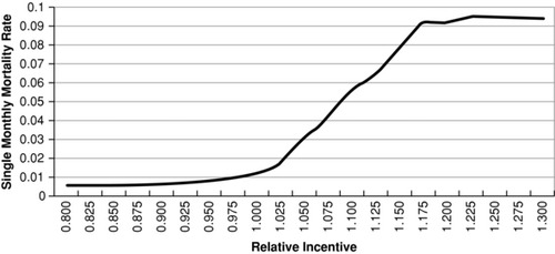
Exhibit 5.2 illustrates the actual refinance curve for Fannie Mae pools based on 10 years of historical data (1999–2009). We see that as the incentive to refinance reaches a ratio of 1.25 the SMM stops increasing. Also, notice that SMM drops off slowly as the refinance ratio falls below 1.0. This illustrates the rate disincentive that movers face. Finally, note that the curve does not approach zero as the incentive falls below 1.0 since there will always be movers.
Other important variables that impact the probability of refinancing include the following:
- Credit score. The lower the credit score of a borrower, the more difficult it is to get a loan, and therefore the lower the probability of prepaying.
- Loan-to-value ratio. A borrower with a high LTV has lower probability of refinancing. One of the biggest drivers of LTV in today's market is housing prices.
- House price appreciation. As home prices increase, the probability that a borrower will refinance to get cash from the house increases. This is called cash-out refinancing, and it was a very common phenomenon from 2005 through the middle of 2007. Similarly, as home prices drop, LTV increases and borrowers are unable to refinance unless they put additional capital into the house.
- Loan size. For a given rate incentive, the higher the loan balance, the greater the probability a borrower will refinance. To the extent that the mortgage payment on a large loan constitutes a greater portion of a borrower's income, a borrower will be relatively more sensitive to mortgage rates.
- Geography. Home price appreciation aside, the condition of the local economy can have a very important differentiating effect on prepayments. Some states, such as those in the Rust Belt,5 have chronic high unemployment, which may suppress prepayments (but increase defaults). State tax policy can also have a significant impact on prepayments. For instance, New York State taxes mortgage refinancing, and as a result, after adjusting for differences in all other factors, prepayments in New York can be as much as 30 percent lower than prepayments in some other states.
In addition to the loan characteristics, there are two other market factors that have been found to significantly impact the probability of prepayment.
1. Media effect. When mortgage rates reach historically low levels, media coverage tends to raise borrower awareness of rate levels, and prepayment activity tends to surge. This was certainly the case in the summer of 2003 when 30-year fixed mortgage rates reached a historical low of 5.21 percent and prepayments on many premium pools surged to 80 CPR. However, it was not the case in 2009 when rates fell as low as 4.7 percent for 30-year fixed mortgage rates, and prepayment activity averaged only 20 to 25 CPR. The 2009 experience reflects lender constraints, since even though a borrower holds an option to prepay her mortgage, she must still meet underwriting standards of the lender to exercise the option.
2. Burnout. When the market mortgage rates fall below the average mortgage rate—weighted average coupon (WAC)—of a pool, the pool will experience an increase in prepayments. However, not all of the loans in the pool will prepay, even if there is a strong incentive to do so. If we assume that the borrowers in the pool are rational, one explanation for this behavior is the existence of one or more unobserved heterogeneities, such as transaction costs. Burnout is the observed effect of these unobserved heterogeneities. When there is a rate incentive to prepay, a self-selection process takes place—pools with low transaction costs prepay. As a result, the average propensity to refinance for the pool declines. The pool is said to have experienced burnout since in the future, if there is a similar incentive to refinance, the prepayment rate for the pool will be lower than it was the first time.
Forecasting prepayments is critical to valuing an MBS when the degree of uncertainty is high. The information that exists is largely inadequate for the task. The agencies primarily report aggregate pool-level data, and while private issuers usually report loan-level information, none of the available data contains demographic information, such as age, gender, employment status, income, occupation, number of children, and wealth of the borrower. These unobserved variables all contribute to forecast bias and error.
In addition to prepayments, the other key determinant of cash flow is defaults. Historically, this has not been a major concern for the loans in agency pools, or even for grade A private-issuer collateral. However, this has all changed in the recent economic downturn, and default modeling has taken on much greater importance. Most of the factors that impact the probability of a loan prepaying also impact the probability of a default. In addition, defaults are also very sensitive to local economic conditions, so the unemployment rate is usually included in a default model.
Prepayment and defaults are the two biggest factors to consider when forecasting cash flow. They are often modeled separately, which is interesting, since the probability of a default is not independent of the probability of a prepayment. Recent modeling initiatives have recognized this dependence, and now the two are often modeled using competing risk models, which calculate the probability of both default and prepayment, recognizing that they are not independent.
Interest Rate Models
The other source of uncertainty in MBS valuation is the interest rate. This is an area where financial engineering has made a major contribution. There are a number of models that can be used to forecast interest rates. We will focus on the Cox-Ingersoll-Ross (CIR)6 model for illustrative purposes and provide a brief summary. A basic knowledge of the interest rate process is crucial to understanding MBS valuation. CIR models the change in the short-term interest rate using the following stochastic differential equation:
![]()
where b is the equilibrium or mean of the short-term rate, a is the rate of reversion to the mean, σ is the standard deviation of the short-term rate, and wt is a Weiner process intended to represent random market risk. This is a mean-reversion model, meaning that if this period's short-term rate is above the mean it will move down over time, and it will move up if it is below the mean rate. This first part of the equation says that the change in the short-term interest rate from t to t + 1 is a function of the distance of the actual short-term rate at time t from its mean, the rate of reversion to the mean, and the change in time. The second part of the equation says that change in the short-term rate is determined by volatility of the rate, the level (square root) of the rate, and a market risk factor. This model is used to forecast the short-term rate from which arbitrage-free bond prices can be derived and the term structure can be calculated.
The interest rate model process has been an area of intense focus for financial engineers. As we will see in the next section, mortgage-backed securities are valued using a simulation process that requires the calculation of hundreds of interest rate forecasts for the term of the bond. It is a process that is feasible only with high-speed, efficient programs.
MBS Valuation
The current state of practice for MBS valuation is the option-adjusted spread (OAS) approach. This is a method that has been in practice since the mid-1980s. In the OAS method, the security price is given, and an interest rate model such as CIR is used to forecast interest rates on many paths over the life of the collateral. A prepayment model is used to forecast cash flows given the interest rate, and OAS is the single spread that makes the average of the discounted cash flows along all interest rate paths equal to the market price of the security. The OAS, which is measured in basis points, is interpreted as the cost of the prepayment option.
The two key inputs into the valuation of an MBS are the prepayment forecast and the term structure of interest rates. The basic valuation equation is:
N = number of simulation paths,
T = number of cash flow periods,
r = short term rate
The typical OAS valuation involves the following three steps:
1. Simulate 500 interest rate paths.
2. Calculate prepayments on each path.
3. Calculate the yield spread of the MBS to London Interbank Offered Rate (LIBOR) (Treasury) curve so the average price across all paths just equals the price of the MBS. This is the expected yield pickup to LIBOR (Treasury) curve, after adjusting for prepayment risk.
The simulation process is computationally intensive. As an example, consider a 30-year fixed-rate pass-through security based on collateral that was just issued. For a 500-path analysis, the OAS method requires the term structure forecast for 359 months along each path and a prepayment forecast for 359 months on each of the 500 paths. For the calculation of duration, this would be done three times, first using the current yield curve to start the simulation process of 500 paths, then shifting the curve up and down 50 basis points, and repeating the process two more times. The magnitude of the computation is also affected by the collateral used to value the security. An agency security might be valued at the pool level or using a more aggregate grouping; in either case, a prepayment forecast and cash flow calculation is required, so if there are 300 pools, the cash flow calculation is done for each pool. In the non-agency world, the collateral is often available at the loan level, and a bond may have 3,000 or 4,000 loans. It is not uncommon to forecast the probability of prepayment and default for each loan at each point in time on each interest rate path (times 3 to calculate duration). This is an area where financial engineering has made an enormous contribution in terms of the development of the analytic methodology, reducing the number of calculations, and generally making sophisticated valuation tools more accessible to a wide group of investors. Today it may take only a minute or two to calculate the duration of a very complex cash flow structure at the loan level.
BEYOND PASS-THROUGHS: COLLATERALIZED MORTGAGE OBLIGATIONS (CMOS)
One of the most important outcomes arising from the development of the OAS valuation tool has been the development of more complex mortgage securities. OAS valuation facilitated the evolution of mortgage-backed securities from simple pass-throughs to a variety of much more complex cash-flow structures called collateralized mortgage obligations (CMOs). A collateralized mortgage obligation is a claim to specific cash flows from a set of underlying mortgages, as opposed to a mortgage pass-through, which is a claim to a pro rata share of all principal and interest payments (less a servicing fee) from the underlying mortgages. The CMO market evolved because there was often a mismatch between the cash flow characteristics of pass-throughs being traded in the secondary mortgage market and the needs of investors. For instance, in the early days of the MBS market, investors with a need to hedge a liability with a two-year duration might have difficulty finding an out-of-the-money pass-through with a matching duration. The first CMO, which was issued by Freddie Mac in 1983, was specifically designed to address investors’ need for greater variability in duration. Additional types of CMOs, designed to offer investors varying levels of exposure to an assortment of risks, soon followed. Today CMO issuance is over $1 trillion per year.
In the most general sense, CMOs use predetermined rules to allocate the principal and interest payments of an underlying set of mortgages to different tranches. The result is a set of bonds with cash flow patterns and risk exposures that can be very different from pass-throughs, and much more suitable to the heterogeneous preferences of investors. Financial engineering has played a very important role in the development of the CMO market, as the techniques for applying the rules, and valuing the tranches, are a computationally intensive application of fixed-income valuation principles.
The earliest CMOs, called sequential bonds, were designed to address the duration mismatch problem. Sequential bonds divide the principal payments from the underlying mortgage collateral into classes that amortized sequentially. For instance, the Class A tranche may pay principal for the first five years while the other three tranches do not make any principal payments. At the end of five years, Class A is fully amortized and the Class B tranche begins to pay principal, which may also amortize over five years. This sequential process continues until the remaining classes are paid off. Thus, the different tranches provide investors with an array of mortgage-backed securities to choose from, each with a different duration. It is important to note that the actual principal payments depend on both the amortization schedule and the actual level of prepayment and default activity. For instance, if prepayments decrease, the duration of all classes in the sequential bond will increase. Sequential bonds satisfy a need for variation in duration, but still expose investors to prepayment risk. The prepayment risk of a sequential bond varies across tranches, and requires an OAS methodology to size and value.
In the mid-1980s, several other types of CMOs were developed that not only provided investors with an array of durations to choose from, but also provided varying levels of exposure to prepayment risk. We will briefly discuss several of these bonds to get a sense of the design and complexity. The planned amortization class (PAC) structure was designed to provide investors with prepayment protection. The PAC structure is composed of two basic types of bonds: the PAC bond and the support bond. The principal payment schedule of the PAC bond is defined as the minimum cash flow associated within a band of prepayment rates. The PAC bond maintains its scheduled principal payments through the use of a support bond. When prepayments are fast, the support bond pays off at a faster rate, allowing the PAC bond to maintain its principal schedule. When prepayments are slow, principal payments to the support bond are delayed so that the PAC schedule can be met. PAC and support bonds are also amortized sequentially to create tranches with different maturities. While the PAC bond does not guarantee principal payments, even if the prepayment rates stay within the predetermined bounds, it does provide limited exposure to prepayment risk, and consequently provides some stability to principal payments. There are a number of different types of PACs that offer different degrees of prepayment protection.
Unlike the sequential and PAC structured bonds, which alter duration and exposure to prepayment risk by restructuring principal payments, floater and inverse floater CMOs are used to create tranches with varying risk exposures by changing the coupon rate. The floater/inverse floater is created by splitting a fixed-rate CMO into two pieces (floater and inverse floater) that amortize simultaneously and have variable rates. The floater has a coupon rate that resets periodically and is calculated using an index (often the one-month LIBOR) plus a margin or spread. The floater rate typically has a lifetime cap and floor, and often has an intermediate cap and floor. The inverse floater has a coupon rate that resets in the opposite direction of the floater and also has caps and floors. A floater/inverse floater structure can be produced from another CMO structure, including a PAC and a sequential bond.
Another important set of CMOs developed in the mid-1980s are the interest-only (IO)/principal-only (PO) bonds (or strips, as they are commonly called). As the name suggests, the IO receives 100 percent of the interest payments from the underlying collateral and the PO receives 100 percent of the principal payments. IOs have negative duration, meaning that when interest rates fall their prices decrease. IO prices are very sensitive to interest rate changes, since a drop in the interest rate will trigger prepayments, resulting in a permanent loss of cash flow. IOs and POs derived from agency collateral trade in a very large, liquid market.
THE NON-AGENCY MARKET
The non-agency (private issue) market originated as a market for loans that were not eligible for securitization by the agencies. Non-agency share of issuance was negligible in the 1980s but grew steadily, reaching 10 percent in 1996 and peaking at 43 percent in 2006. Share of issuance has dropped off considerably since 2006 as the housing market declined. Developments in financial engineering played an important role in the growth of the non-agency market. Non-agency collateral is much more heterogeneous than agency collateral, making the valuation process more information-intensive. Valuation and analysis are typically done at the loan level, as opposed to agency deals, which do not provide loan-level information. In addition, non-agency bond structures tend to be more complex because they incorporate credit enhancements not present in agency CMOs.
There are several fundamental differences between agency and non-agency collateral, bonds, and market structures. First, unlike agency bonds, which are guaranteed by the U.S. government either explicitly (Ginnie Mae) or implicitly (Fannie Mac, Freddie Mac), non-agency bonds do not have a guarantee of timely payment of principal and interest. Non-agency CMO issuers have attempted to compensate for this additional level of credit risk by incorporating a credit tranche structure into their CMOs.7
There are also important differences in the quality of agency and non-agency collateral. While many of the loans that are bundled into non-agency CMOs meet agency underwriting standards, there are also loans that do not. For instance, a borrower's credit score may be too low to qualify for an agency loan, or the borrower may not provide the necessary documentation to qualify for an agency loan. A large portion of the non-agency loans do not have full documentation, meaning that the borrower does not provide written proof of employment, income level, and/or net wealth. For these partial-documentation loans, the lender accepts a written, unverified statement of employment and/or income from the borrower in lieu of verification. These loans have become known as liar loans. Another important difference in loan quality is that non-agency loans can have an LTV that exceeds 80 percent, whereas agency collateral cannot. At the height of the recent housing boom, some non-agency loans originated with 100 percent financing. Finally, agency and non-agency loans can differ by loan size. The non-agency issuance is not restricted by the conforming balance limit. As a result there is an entire market segment (called jumbos) of conventional loans that are ineligible for agency securitization.
Up until the early 1990s, a non-agency deal could contain any type of loan, regardless of whether it was a jumbo loan with a high credit score and a low LTV, or a conforming balance loan with a low credit score and no documentation. The heterogeneous nature of the underlying collateral of non-agency bonds restricted its appeal to investors. Low- and high-quality collateral generally appeal to investors with very different risk preferences. Heterogeneity also made the bonds difficult to value. Factors such as loan size, credit score, LTV, and documentation type are each important determinants of prepayment and default risk. The ability to produce a reasonable forecast of expected cash flow requires loan-level data processing, models, and analysis, which is an effective barrier to entry. Segmenting the market was a logical step toward increasing the appeal of non-agency bonds to investors.
In 1993, private banks began issuing CMOs with credit grades based on the characteristics of the underlying collateral. The three main categories that were created and are still in use today include jumbo prime, which is comprised of loans that exceed the conforming balance limit but are otherwise equivalent in quality to agency loans; Alt-A, which are grade A bonds backed by loans that have balances below the conforming limit but do not meet agency underwriting standards because the credit score is too low, the LTV is too high, or the borrower failed to provide full documentation; and subprime, which are grade B and grade C bonds backed by poor credit-quality loans, such as a loan with a low credit score, high LTV, and no documentation. The definitions are not hard-and-fast, but the segmentation provided a degree of homogeneity that facilitated valuation and generally increased investor appeal.
Even with credit segmentation, the characteristics and creditworthiness of non-agency collateral tend to be much more heterogeneous than agency collateral, so the models used to forecast prepayments and defaults tend to be much more complex. Analysis and valuation of non-agency bonds typically use loan-level information, whereas agency bonds are valued at the pool level or a more aggregate level since virtually no useful loan information is available from the agencies. As a result, the valuation process for non-agency bonds tends to be computationally more demanding than agency valuation. Many investors in the non-agency market recognize the need to analyze deals at the loan level, and have the capability to do so.
The rapid growth in non-agency issuance share, from 10 percent in 1996 to 43 percent in 2006, can be attributed in part to the segmentation of the market in the early 1990s. It can also be attributed to a significant increase in the origination of so-called affordability products such as adjustable-rate mortgages (ARMs), hybrid ARMs, nonamortizing (interest-only loans) loans, and option ARMs, all of which were designed to provide borrowers with lower monthly loan payments, but typically just do so temporarily. In 2001, approximately 75 percent of all Alt-A originations were fixed-rate mortgages. By 2005 only about 20 percent were fixed-rate mortgages.8
In the five-year period leading up to its peak in 2006, the increase in non-agency issuance was accompanied by a decline in the quality of borrower characteristics. For instance, the percentage of Alt-A loans with full documentation declined from 35 percent in 2001 to 16 percent in 2006. The percentage of Alt-A loans with silent second mortgages increased from 1 percent in 2001 to 39 percent in 2006. (A silent second mortgage is a second mortgage that was not disclosed to the first mortgage lender at origination.) The average LTV on a subprime loan was 86 percent in 2006 compared with 80 percent in 2001.9 Banks were lending money to riskier borrowers, and many of the loans found their way into non-agency CMOs, which, unlike agency CMOs, do not have an implicit or explicit guarantee of timely payment of principal and interest.
Non-Agency CMOs
Because non-agency bonds do not have a credit guarantee, issuers use a senior/subordinate structure to create credit tranches and redistribute credit risk. A common non-agency CMO structure10 is illustrated in Exhibit 5.3. Principal and interest payments flow from the top down, giving the senior tranche, which is typically rated AAA, priority to the principal and interest payments from the collateral. The subordinate tranches have lower credit ratings and may or may not be investment grade. The bottom tranche, often called the junior tranche, may not be rated at all.
Exhibit 5.3 Generic Non-Agency CMO Structure
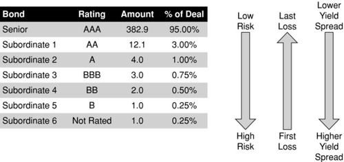
In addition to the top-down flow of principal and interest, the senior tranche is protected by making it the last to incur losses. Losses are allocated from the bottom up, meaning that the lowest-rated tranche is the first to receive principal losses. The subordinate bonds protect the senior bond until their principal is depleted. In Exhibit 5.3 the subordinates will absorb the first $23.1 million in losses before the senior tranche suffers any loss. The relative size of the subordinate tranches dictates the level of protection. The protection afforded by this credit-enhancing structure allows the senior tranche to hold its triple-A rating.
Non-agency CMOs often provide additional credit protection to the senior tranche by allocating the subordinate bond's share of any prepayments to the senior for a fixed time period, often referred to as the lockout period. The lockout period can vary from five to 10 years depending on the type of collateral. For instance, in the case of a CMO backed by 30-year fixed-rate Alt-A mortgages, all prepaid principal may be allocated to the senior tranche for the first five years of the bond's life. This is called a shifting interest structure. It has the effect of increasing subordination over time by making the subordinate bonds larger. Finally, the individual credit tranches in a deal may also be split into sequential bonds, PAC bonds, interest-only/principal-only bonds, floaters/inverse floaters, and other types of structures, which, as we previously discussed, have the effect of shifting prepayment and/or interest rates.
The level of credit protection provided to the senior bonds by the senior-subordinate structure depends on the size or thickness of the subordinate piece. Establishing an appropriate level of subordination for a deal requires an estimate of losses, or mortgage defaults. Statistical models for forecasting the probability of default depend on historical experience. Most models use data from the past 15 years to forecast defaults. The national level of defaults for the period 2007–2009 has been greater than for any other period except the Great Depression. As a result, default models have grossly underforecasted default rates, and subordination levels have in many instances been inadequate to protect the triple-A rating of senior tranches.
FINANCIAL ENGINEERING AND THE FUTURE OF THE SECONDARY MORTGAGE MARKET
The economic downturn has taken its toll on the market for mortgage-backed securities. In 2008, total MBS issuance declined by 35 percent to $1.3 trillion. This is roughly half the level of total issuance in the peak year 2003. There are signs of a recovery for the MBS market as a whole, with total issuance up 40 percent in 2009. But aggregate statistics often tell a misleading story. Agency issuance declined only 5 percent in 2008, and it increased 43 percent in 2009. Non-agency issuance, however, plummeted, declining 95 percent in 2008 and an additional 47 percent in 2009. As a result, the non-agency share of issuance declined in 2009 to a mere 1.3 percent.
Although Fannie Mae and Freddie Mac are in financial straits, the agency market will eventually rebound. The federal government is still committed to a housing policy that helps provide affordable housing. The 2009 federal tax credit for first-time home buyers has stimulated the origination of FHA-insured loans, which are typically securitized by Ginnie Mae. The explicit federal guarantee of the timely payment of principal and interest has increased the demand for Ginnie Mae bonds. Agency CMOs as a whole comprise the highest-quality mortgages. The logic of carving up the cash flows from high-quality loans to create bonds that meet the needs of investors is still sound, and as a result, agency CMOs will always be in demand.
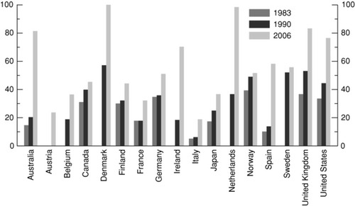
Exhibit 5.4 Mortgage Debt Outstanding (percent of GDP)
Source: IMF. This chart was published in 2008 and can be accessed at: www.imf.org/external/pubs/ft/weo/2008/01/c3/Fig3_1.pdf.
The future of the non-agency market will depend on its ability to adapt to the new economic reality. Credit risk has proven to be much greater than ever anticipated, and the rejuvenation of the non-agency CMO market will depend on the ability of issuers to structure CMOs that provide greater protection. For instance, the level of subordination in a deal will probably have to be much higher than it has been in the past. In the future, a 5 percent cushion of subordination will probably be deemed too low to protect a senior tranche. In addition, the valuation process will have to make greater use of loan-level data. Investment decisions will require improved methods for evaluating the multiple dimensions of risk in a non-agency CMO, and financial engineering will necessarily play a key role.
A NOTE ON THE GLOBAL GROWTH OF THE MORTGAGE MARKET
The enormous growth of mortgage lending experienced in the United States over the past few decades is not unique. Similar patterns have been experienced throughout the world. Exhibit 5.4 depicts the size of the mortgage markets for a number of countries for select years.
NOTES
1. The prevalent fixed-rate 30-year mortgage of today was rare in the 1930s. Many mortgages were balloon loans where the entire principal payment was due at one time, usually three to five years after origination.
2. The investor receives principal plus interest, less a fee paid to the mortgage servicer for collecting payments from the borrower.
3. One major exception to this characterization, as we will see, relates to differences in credit risk.
4. Some additional determinants often included in a turnover model are credit score, loan-to-value ratio at origination, slope of the yield curve at origination, and spread between the borrower's mortgage rate and the average mortgage rate at origination.
5. The Rust Belt includes parts of the northeastern United States, the mid-Atlantic states, and portions of the eastern midwest.
6. The CIR model was one of the first internally consistent term structure models. See Rebonato (2004) for a survey of interest rate models.
7. Credit enhancement and non-agency CMO structure are discussed in the next section.
8. See Kramer and Sinha (2006).
9. Loan performance in Ashcraft and Schuermann (2008).
10. This structure is common for CMOs backed by non-agency Alt-A and jumbo prime collateral. CMOs backed by subprime mortgages often provide additional credit enhancement through excess spread and overcollateralization.
REFERENCES
Ashcraft, Adam A., and Til Schuermann. 2008. “Understanding the Securitization of Subprime Mortgage Credit.” Federal Bank of New York Staff Report No. 318.
Fabozzi, Frank J. 2005. The Handbook of Mortgage-Backed Securities. 6th ed. New York: McGraw-Hill.
Gorton, Gary. 2008. “The Panic of 2007.” Unpublished paper prepared for the Federal Reserve Bank of Kansas City, Jackson Hole Conference, August.
Kramer, Bruce, and Gyan Sinha. 2006. Bear Stearns Quick Guide to Non-Agency Mortgage Backed Securities. Bear Stearns, September.
McDonald, Daniel J., and Daniel L. Thornton. 2008. “A Primer on the Mortgage Market and Mortgage Finance.” Federal Reserve Bank of St. Louis Review (January/February 2008): 31–46.
Rebonato, Riccardo. 2004. “Interest Rate Term-Structure Pricing Models: A Review.” Proceedings: Mathematical, Physical and Engineering Sciences 460:2043, 667–728.
ABOUT THE AUTHOR
Bruce McNevin is the managing director of Mortgage Research at The MidWay Group, a hedge fund specializing in mortgage-backed securities. His primary responsibilities include directing development of mortgage prepayment models and conducting relative value research on MBSs. Dr. McNevin holds a PhD in economics from the City University of New York.