
Chapter 4
The Fixed Income Market
Fixed Income Market Snapshot
History: The interest rate derivatives markets began to develop in the late 1970s. Early on, the instruments that were traded were mainly used for risk management purposes by corporations exposed to interest rate fluctuations. However, the instruments were soon applied by other types of users for their hedging and investment needs. Eventually, the early derivatives led to the development of more complex, structured financial products. For these reasons, interest rate derivatives eventually became the largest segment, by far, of the global derivatives markets.
Size: The interest rate market is the largest component of both over-the-counter (OTC) and exchange-traded derivatives. The size of the OTC interest rate derivatives market has grown from $50 trillion at the end of 1998 to about $449 trillion at the end of 2009, while the exchange-traded derivatives side has evolved from $12.6 trillion in 1998 to $67 trillion in 2009.
Products: Over-the-counter products include interest rate swaps (either fixed-for-fixed or fixed-or-floating swaps), caps, floors, collars, corridors, swaptions, warrants, forward rate agreements (FRAs), and bond options. Exchange-traded instruments consist of a variety of interest rate futures on Treasury bonds and bills, Federal Funds, Eurodollars, and EuroYen.
First Usage: In 1975, the Chicago Board of Trade created the first interest rate futures contract based on Ginnie Mae mortgage pass-throughs. Though it met with initial success, the contract eventually died. The first successful interest rate futures contract, a 90-day U.S. Treasury bill futures contract, was produced by the Chicago Mercantile Exchange in the same year. One of the first interest rate swaps was transacted in 1982 by the Student Loan Marketing Association (Sallie Mae) in a successful effort to convert fixed-rate payments for its intermediate-term debt to floating rate payments indexed to the three-month Treasury bill rate.
Selection of Famous Events:
1989: The British local government of Hammersmith and Fulham Borough Council defaulted on about $10 billion worth of interest rate swaps and options contracts when rising interest rates reversed their income flow. Eventually, British courts ruled that Hammersmith and Fulham, as well as other local government councils that also participated in derivatives trading, had exceeded their legal powers by entering into the interest rate derivative contracts
1994: Procter & Gamble and Bankers Trust Company entered into two highly leveraged interest rate swaps, which made them more susceptible to market swings. The products were structured to pay off handsomely for P&G if interest rates continued to fall. They did not. A sudden increase in interest rates resulted in P&G incurring a $157 million loss.
1994: Air Products & Chemicals also entered into a derivative transaction with Bankers Trust. It wanted to lower its interest costs on $1.8 billion of loans and bonds and use the swaps to convert its fixed, high-interest rate obligations to lower variable rates. To achieve this, the company purchased five leveraged interest-rate swap contracts. When rates rose, the company suffered a pre-tax loss of $96.4 million.
Best Providers (as of 2009): The Best Interest Rate Derivative Provider, as ranked by Global Finance magazine, is JP Morgan in North America, Standard Chartered in Europe, and Royal Bank of Scotland (RBS) in Asia.
Applications: Some of the ways in which interest rate derivatives can be used include hedging against exposure to fluctuations in interest rates, mitigating cash flow volatility, lowering funding costs, and arbitraging debt price differences in the capital markets.
Users: Investors in interest rate derivatives include corporations (both financial and non-financial), government agencies, and various types of international institutions.
INTRODUCTION
Global fixed income markets cover a broad array of securities and vary considerably in their structure and complexity. Such fixed-income securities represent a significant portion of the asset allocation mix of institutional investors. They offer proprietary traders and hedge fund managers large and liquid markets to implement relative value, arbitrage and directional strategies. They provide investors, directly and indirectly, a wealth of information on the health of financial markets and macroeconomic conditions.
Over the past 10 years, investments in fixed income have outperformed investments in equities. From September 2000 to September 2010 the annual return on S&P 500 index was –1.4 percent and 1.6 percent for the MSCI Developed World (except the United States). In contrast, the Barclays US Corporate bond index was up 6.9 percent, the Barclays U.S. High Yield bond index returned 9.4 percent and the return on Barclays Euro Corporate bond index was 9.4 percent. In emerging markets, sovereign debt and equities performed equally well. The MSCI Emerging Market stock index was up 11.2 percent, while the Barclays Sovereign Debt index was up 11 percent. Today, as global economies recover from the 2008 credit crisis, the fixed income markets are entering a period of uncertainty and are poised for remarkable change.
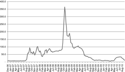
On the demand side, after the collapse of the financial markets in 2008, investors have shown an insatiable appetite for fixed income securities. According to the Investment Company Institute, between January 2007 and July 2010 a total of $698 billion flowed into U.S. bond mutual funds while $153 billion flowed out of equity funds during the same period. Around 70 percent of the bond inflow took place since September 2008. These flows are depicted in Exhibit 4.1.
Exhibit 4.1 Cumulative Long-Term U.S. Mutual Fund Flows, January 2007–July 2010
Source: Investment Company Institute (http://www.ici.org).
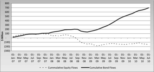
The desire for income in a low global interest rate environment, disappointment with performance of equity markets over the last several years, concerns about high risk with equity investment due to the slowdown in economic growth, and a growing fear of deflation have all contributed to this flood of money into fixed income markets. Moreover, with an aging population in the developed world, it is likely that the flows will persist, as the retiring population directs more of its investment to fixed income markets. Toward this goal, pension funds will further increase their allocation to these markets as they pursue liability-driven investments.
On the supply side, an entirely different dynamic is playing out. The massive deleveraging of the financial system and corporate balance sheets is resulting in a decline in the supply of fixed income securities. Several financial products that were manufactured during the credit bubble will not survive. Partially offsetting this is a flood of new government debt securities issued to fund massive budget deficits brought on by efforts to stimulate the economy. The challenges of reinvesting debt that is rolling over, the gap between the supply and demand for securities, and concerns about emerging sovereign debt crises in the developed economies are fundamentally altering the landscape of fixed income markets. In the near term, it is likely that the money flows into some of the corners of the fixed income markets (such as emerging markets) will reach levels beyond the size of these markets, thus potentially causing another bubble and elevating liquidity risks. Market price and yield relationships within the fixed income markets that have been relatively stable for decades, and never been in doubt, are beginning to unravel. The 30-year U.S. dollar interest rate swap spread has turned negative, something not observed in the past. It is likely that the rationale for several market relationships will be revisited, and a new investment paradigm may emerge. Some of the emerging market economies are in a strong fiscal position while the developed markets struggle with deficit and debt. The credit spreads between the sovereign debt of emerging and developed markets will need to recalibrated. Regulatory reforms, reduced risk-taking by dealers, and the exit of many participants, have all affected market liquidity and trading volume. In the past, the behavior of the fixed income markets has been defined by interest rate levels and interest rate volatilities. This will continue, but, as we go forward, it will be just as important to understand and closely watch investor perceptions of demand and supply to fully evaluate the risks and returns in the fixed income markets.
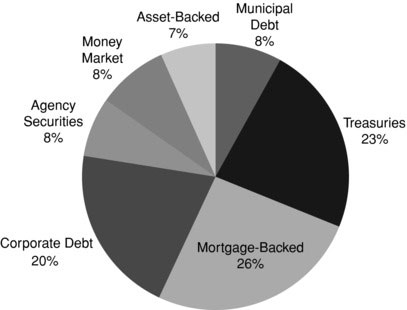
The fixed income markets can be divided into cash and derivative markets. The cash side of the U.S. fixed income market is by far the largest debt market globally. U.S. Treasury debt and mortgage-backed securities (MBS) combined constitute approximately 50 percent of the cash market. Corporate debt comprises about 20 percent. Exhibit 4.2 depicts the composition of the cash market at the end of the first quarter of 2010.
Exhibit 4.2 U.S. Bond Market, Q1 2010 Total Debt: $35 Trillion
Source: SIFMA (http://www.sifma.org).
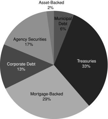
New U.S. debt issuance for the full year 2009, shown in Exhibit 4.3, follows a similar break-down with U.S. Treasuries and MBS dominating the market.
Exhibit 4.3 U.S. Bond Issuance, 2009 Total Issuance: $6.7 Trillion
Source: SIFMA (http://www.sifma.org).
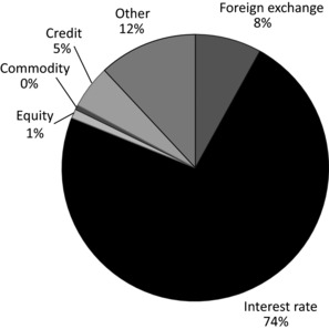
The derivatives side of the fixed income market includes both instruments that trade on exchanges and instruments that trade in over-the-counter (OTC) dealer markets. Fixed income derivatives represent the largest part of the total derivative market, with much of the trading activity taking place in the OTC markets. At the end of 2009, the total notional value of all outstanding OTC derivative contracts stood at $614 trillion. Interest rate derivatives made up 73 percent of this. This is depicted in Exhibit 4.4.
Exhibit 4.4 Over-the-Counter Derivatives Market, 2009 Total Outstanding: $614 Trillion
Source: BIS (http://www.bis.org).
This chapter is an introduction to the fixed income markets. Section 2 reviews the cash component of the fixed-income securities markets. Agency and mortgage-backed securities are excluded as they are a topic of discussion elsewhere in this book. Fixed income derivative products are covered in section 3. Sections 4, 5, and 6 presents some key topics related to analysis of fixed income securities. In section 7 a few trading strategies are outlined.
THE CASH MARKETS
Treasury Debt
The roughly $13 trillion U.S. Treasury debt market is the largest fixed income market in the world. This market represents debt issued by the U.S. government, and the payment is guaranteed by the taxing authority of the United States. It is the principal means of financing the U.S. federal deficit and refinancing maturing debt.
Ownership and Make-Up: Historically, due to the reserve currency status of the U.S. dollar (hereinafter referred to as USD), U.S. Treasuries have established a unique status as a storehouse of value. The USD is considered a safe haven, with investors ranging from central banks to pension funds to individual investors. Approximately 60 percent of the debt is public-marketable, with the rest accounted for by public non-marketable and intra-governmental holding that includes the U.S. Federal Reserve and the Social Security Trust Fund.
As of December 2009, approximately 30 percent of total outstanding U.S. Treasuries were held by foreign and international entities. Another 15 percent were held by Pension Funds, Insurance Companies, Mutual Funds, and State and Local Governments.
Among foreign and international entities, China and Hong Kong are the largest owners, with 25 percent of ownership. They are followed by Japan at 20 percent and the United Kingdom at nine percent. BRIC nations (Brazil, Russia, India, and China), along with Hong Kong, Japan, and the United Kingdom, make up 62 percent of the foreign U.S. Treasury ownership.
The eight trillion dollars of public marketable Treasury securities can also be categorized by maturity as T-bills, T-notes, and T-bonds, plus an inflation-indexed product called Treasury Inflation-Protected Securities (TIPS). When looked at this way, the market consists of:
T-Bills—22 percent
T-notes—61 percent
T-bonds—10 percent
TIPS—7 percent
T-bills are short-term securities sold at a discount, whereas notes and bonds are interest-bearing obligations that pay a coupon semi-annually. TIPS also pay interest semi-annually, but the principal is indexed to the CPI-U. The CPI-U is the non-seasonally adjusted U.S. City Average All Items Consumer Price Index for All Urban Consumers, published monthly by the Bureau of Labor Statistics of the U.S. Department of Labor. In case of deflation, the principal is adjusted downwards resulting in a lower interest payment, but at maturity the Treasury guarantees repayment of the original principal if the adjusted principal falls below the original principal.
New Issuance: Treasuries are regularly issued via a cycle of announcements followed by auctions. The 4-week, 13-week, and 26-week Treasury bills are auctioned each week while the 52-week bills are offered every four weeks. The 2-year, 5-year, and 7-year notes are normally announced in the second half of the month and auctioned a few business days later. The 3-year and 10-year auctions are announced during the first half of the month. More specifically, the 10-year is usually announced during the months of February, May, August, and November. The 5-year TIPS are auctioned in April (reopened in October), 10-year TIPS are auctioned in January and July (reopened in March, May, September, and November), and 30-year TIPS are auctioned in February (reopened in August). A reopened Treasury has the same coupon rate, payment date, and maturity date but a different price.
The Treasury auction process begins with the announcement of the auction for a specified amount. The auction process determines the coupon rate and the issue price of the debt. Immediately following the auction announcement, dealers begin to trade the security on a when-issued basis. Securities purchased and sold on a when-issued basis settle on the issue date of the security, unlike normal secondary market transactions in Treasuries that settle in one business day. When-issued trading reduces uncertainty, enhances transparency, and facilitates price discovery. Potential bidders use the information to bid at the auction. Prior to 1992, Treasury auctions followed a multiple-price format, wherein each competitive bidder paid prices computed from their bid yield. However, in 1992, the U.S. Treasury adopted a single-price format for the auction.
Market participants submit either one or more competitive bids specifying the yield and quantity, or a noncompetitive bid specifying the quantity they are willing to purchase at the price established by the competitive bidders. The Treasury Department limits each bidder to 35 percent of the offering, less the bidder's “reportable net long position.”
The Treasury, after subtracting noncompetitive bids, accepts competitive bids in the order of increasing yield until all securities being offered are exhausted. The highest accepted yield, called the “stop,” establishes the single clearing price. Bids below the stop are filled in full, at the stop are filled prorated, and above the stop are rejected. The coupon rate is set to the highest level, in 1/8th percent increments, so as to not exceed a price of 100 percent.
Auctions for T-bills are similar except that competitive bids are in terms of discount rates. The auction market underwent several changes in 1992 after the discovery of a significant violation of bidding rules by Solomon Brothers. The firm bid inappropriately, such that it gained as much as 86 percent of a new issue.
Exhibit 4.5 reports the result from a recent 10-year auction held on August 11, 2010. FIMA stands for Foreign and International Monetary Authority and SOMA is the Federal Reserve System's Open Market Account. The bid/cover ratio, which is the ratio of total bids (excluding SOMA) to the total amount sold, was 3.04. The bid/cover ratio for the 10-year U.S. Treasury over the last 10 years has ranged between 3.7 and 1.2, with an average of around 2.4. The bid/cover ratio is a gauge of market demand for the debt and has taken on an added importance since 2008.
Exhibit 4.5 Results of 10-Year U.S. Treasury Auction
| Treasury Auction Results: August 11, 2010 | ||
| Issue Date | 16-Aug-10 | |
| Maturity Date | 15-Aug-20 | |
| Original Issue Date | 16-Aug-10 | |
| Coupon Rate | 2.625% | |
| High Yield | 2.73% | |
| Allotted at High | 10.57% | |
| Price | 99.087 | |
| Median Yield | 2.67% | |
| Low Yield | 2.66% | |
| Tendered | Accepted | |
| Competitive | $72,820,240,000 | $23,824,219,500 |
| Noncompetitive | $125,810,700 | $125,810,700 |
| FIMA (Noncompetitive) | $50,000,000 | $50,000,000 |
| Subtotal | $72,996,050,700 | $24,000,030,200 |
| SOMA | $1,437,197,100 | $1,437,197,100 |
| Total | $74,433,247,800 | $25,437,227,300 |
| Tendered | Accepted | |
| Primary Dealer | $49,067,000,000 | $10,375,725,500 |
| Direct Bidder | $9,936,000,000 | $2,532,513,000 |
| Indirect Bidder | $15,817,240,000 | $10,915,981,000 |
| Total Competitive | $72,820,240,000 | $23,824,219,500 |
While, traditionally, the U.S. Treasuries have held significant weight in the asset allocation of investors globally, the future is more uncertain. The U.S. Treasury's debt has increased exponentially in the last few years; more than 50 percent since December 2006. This has been the result of U.S. central bankers’ and policy makers’ aggressive monetary and fiscal policies to counter the economic fallout from the 2008 credit crisis. The U.S. Treasury debt to GDP (see Exhibit 4.6) is 100 percent. This alarming rise in debt has led many leading investment professionals to question the status of U.S. Treasuries as a safe haven and to question its AAA credit rating. Any change in demand for U.S. Treasuries or investor perception will have enormous implications for fixed income markets, given the dominance of the U.S. Treasuries in the market. Also, the purchase and sales decisions of a few foreign and international entities will have significant impact on the Treasury market given the concentration of international ownership.
International Debt
The international debt market can be classified into domestic bonds, foreign bonds, and Eurobonds. Domestic bonds are issued by domestic borrowers in their local currency and sold locally. The foreign bond market is debt issued by foreign borrowers in domestic currency and sold domestically. An example of the latter would be a Japanese issuer selling a bond in the United States that is denominated in USD.
The foreign bonds traded in the foreign bond markets constituted a significant portion of the international bond market until a few decades ago. Foreign bond issuers typically include national governments and supranationals. For example, in September 2010, BNP Paribas went to the Japanese capital market with a 5-year 1.04 percent JPY 59.3 billion bond issue (referred to as a Samurai bond). Yankee bonds are foreign bonds issued in USD in the U.S. market.
Eurobonds differ from the others in that they are not sold in any particular domestic bond market. Eurobonds are denominated in a currency not native to the country where they are issued. So if a Eurobond is denominated in the U.S. dollar, it would not be sold in the United States. The 5-year USD 2 billion 3.625 percent Russian debt issuance in April 2010 is an example of a Eurobond.
Historically, the pound Sterling used to play a key role in international trade. This predominance ended following the Bretton Woods conference in 1944 and the subsequent Sterling crisis. Today the USD is the largest reserve currency, followed by the Euro, the pound Sterling, and the Japanese yen. These currencies dominate the global foreign exchange markets and also make up much of the international debt market. Exhibit 4.7 shows marketable government debt for the top 25 OECD countries.
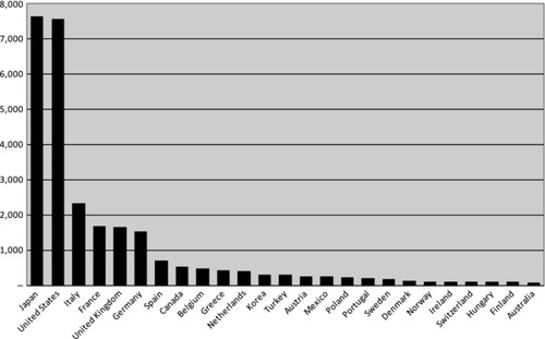
U.S. Treasuries and Japanese Government Bonds (JGB) dominate the government debt market, followed by Italy, France, UK, and Germany.
The Italian BOTs are short-term bonds with maturity up to one year. CTZs are zero coupon Italian bonds with two-year maturities. The Italian Treasury bonds with maturities of 3, 5, 10, 15, and 30 years are called BTPs. The Italian Treasury also issues bonds indexed to the Euro-zone inflation rate and are called BTP Euro i notes. These bonds are issued with 5-, 10-, 15-, and 30-year maturities.
OATs, BTANs, and BTFs are the French long-term, medium-term (two to five years) and short-term bonds. Maturity and coupon dates of fixed rate OATs are either 25th April or 25th October. In addition, there are inflation-linked OATs indexed to a French consumer price index (excluding tobacco) or to the Euro-zone inflation index.
The largest share of the UK government's debt are conventional gilts described by a coupon rate, a maturity date, and paid semi-annually. Index-linked gilts are the largest part of the gilt market after conventional gilts. They also pay a coupon semi-annually, but the principal is adjusted according to the UK Retail Price Index.
The German bond market consists of Bunds, Bobls, and Schatz. Bund maturities range from 10 to 30 years. Bobls are five-year notes and Schatz refers to the two-year notes. Another significant German debt market is the Pfandbrief. The total Pfandbrief outstanding, as of 2009, was EUR 719 billion. These are medium- to long-term covered bonds issued by German credit institutions (Pfandbriefbanken). The bonds are secured or “covered” by a pool of eligible cover assets, such as mortgages or public sector loans. Pfandbrief debt issues are governed by the German Pfandbrief Act which imposes strict legal requirements on the quality and overcollateralization of assets.
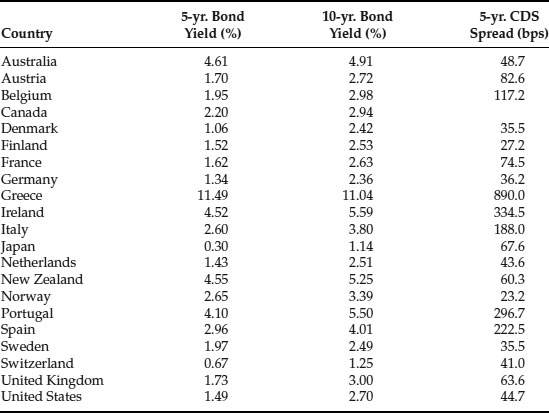
The Eurozone, with a common currency and the European Central Bank administering the monetary policy, is the largest liquid government debt market outside the United States. However, the government debt of Eurozone countries is far from uniform. There is substantial economic disparity among these countries, resulting in considerable differences in yield and trading activity of the debt of these countries. The market's perception of an issuer's credit quality is best illustrated by the price (called a spread) of purchasing credit protection on that debt by way of a credit default swap (CDS). Exhibit 4.8 illustrates comparative spreads for the debts of different countries.
Exhibit 4.8 Major Developed Market Government Bond Yield and CDS Spreads
Source: Bloomberg Finance L.P.
Municipal Debt
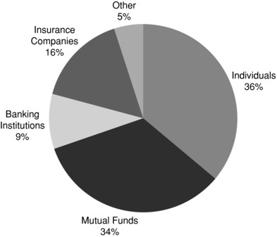
The $2.8 trillion U.S. municipal bond market consists of taxable and tax-exempt bonds. U.S. individuals and mutual funds (money market funds, bond funds, and closed-end funds) constitute the largest owners. This is depicted in Exhibit 4.9. Further, the municipal bonds can be classified as General Obligation (GO) bonds and revenue bonds. GO bonds are secured by the unlimited taxing power of the state and local governments. This means that if the municipality encounters financial problems it will need to raise taxes to repay the bondholders. In many states, such as California, the constitution demands that the bondholders of state-backed debt be paid back first before using money for any other purposes. Local governments back their GO debt with taxes from property. GO bonds are generally considered the safest form of municipal debt. The interest and principal repayments on the revenue bonds are backed by the revenues from the project being financed.
Exhibit 4.9 Municipal Debt Ownership Total Debt Outstanding: $2.8 Trillion
Source: SIFMA (http://www.sifma.org), with data from the Federal Reserve System.
Examples of revenue bonds are Airport, Hospital, University, Industrial Development, Water and Sewer, and Toll Road. Unlike GO bonds, the revenue bonds are more risky as they are only supported by the revenues from the project. Revenue bonds issued for essential services such as water, sewer, and power are generally considered safer than non-essential service bonds. In 2009, $221 billion of municipal bonds were issued, 40 percent GO and 60 percent revenue bonds. The U.S. municipal bond market is entirely a domestic market. The primary motivation to hold this debt is the exemption of U.S. federal taxes on the interest payment. The state taxes may also be exempt if the investor is a resident of the state issuing the bonds. Due to the tax-exempt status of municipal bonds they generally pay a lower interest rate compared to corporate bonds. The attractiveness of the debt is therefore a function of the marginal tax rate of an investor and other U.S. tax regulations.
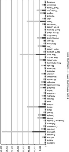
Taxable municipal bonds had made up a very small fraction of total municipal bond issuance. However, this has changed since 2009 with the introduction of Build America Bonds (BABs). BABs are taxable municipal bonds that were authorized under the America Recovery and Reinvestment Act of 2009 and signed into law in February 2009. BABs can be direct pay or tax-credit BABs. They offer states and local governments an alternative to issuing tax-exempt municipal bonds. They cannot be used for refunding, working capital, private activities, or 501(c)(3) tax-exempt organizations. Since the interest on BABs is taxable, the interest rates are higher than tax-exempt municipal bonds. The federal government makes up for the lack of benefits associated with tax-exemption. In the case of direct pay BABs, the federal government provides a cash subsidy payment equal to 35 percent of their interest costs to issuers of BABs. The investors of tax-credit BABs receive a federal income tax credit equal to 35 percent of their BABs interest income. Since 2009, $130 billion of BABs have been issued. Most issuances have been direct pay BABs. California, Illinois, New York, and Texas have been the largest BABs issuers. This is depicted in Exhibit 4.10.
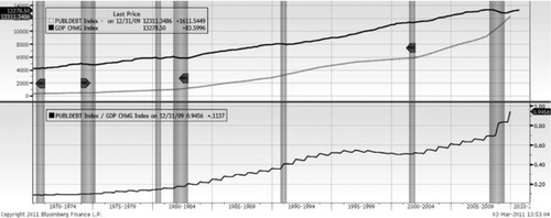
While U.S. Treasury securities have generally been considered a proxy for a risk-free asset, municipal bonds are not. Historically, municipal bond defaults have been low, and their ultimate recovery high. No state has defaulted on state GO municipal bonds since the Civil War. For instance, in the most notable default in 1994 by Orange County, California, the investors were paid back 100 percent with interest within 18 months. Most defaults were linked to poor debt management and financing arrangements. The default of municipal bonds was less of a consideration for the investor in the past, since many issuers insured their bonds against default with private insurance companies, such as MBIA, Ambac, or FIGIC. However, the municipal bond market is undergoing a regime shift following the 2008 credit crisis. With the demise of many bond insurers and the difficult fiscal position of many states, it is no longer a pure play on taxes and interest rates. The likelihood of a further increase in municipal bond defaults is making this a testing market for inexperienced investors. The current $3-billion-a-year collective default rate is three times the historic collective default rate of $1 billion or less a year going back to 1983. Bloomberg Businessweek reported that thirty-five municipal bond issues, totaling $1.5 billion, defaulted in 2010. It was 194 issues, totaling $6.9 billion, in 2009. (Default totals for some earlier years are depicted in Exhibit 4.11.) Macroeconomic conditions, credit analysis, and legal structure will all be equally important to evaluate the risk and rewards in this market.
Exhibit 4.11 Municipal Bond Default
Source: “Muni Bond Default Parade Plays On,” January 15, 2009, Forbes.com.

Repurchase Agreements
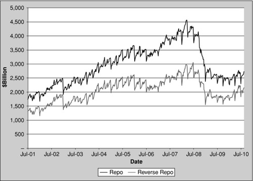
A repurchase agreement or repo is a sale of a security combined with an agreement to repurchase the same security at a later date. A reverse repo is the other side of the transaction. Normally the repurchase price is higher than the sale price, and the difference represents the interest rate, known as the repo rate. A repo is thus similar to a collateralized lending, with the caveat that the title passes at the opening and the closing of the transaction. The passing of the title reduces counterparty risk for the lender of the cash against default events. While statistics on the total repo market are difficult to find, some estimate the U.S. repo market to be around $12 trillion. The Federal Reserve Bank of New York (FRBNY) reports the repo and reverse repo financing by primary dealers (see Exhibit 4.12).
Exhibit 4.12 Primary Dealer Financing: Repo and Reverse Repo
Source: Federal Reserve Bank of New York.
Repos can be overnight, term (with a specified end date), or open (with no end date). They can also be classified as General Collateral (GC) or Specified Collateral (sometimes called specific collateral). In a GC, the lender of cash is willing to accept any of a variety of Treasury and other related securities as collateral. A specified collateral repo requires the borrower of cash to post a specific security as collateral. The repo rate for a specified collateral repo is always lower than the GC repo, and can even be negative if the security posted as collateral is in short supply.
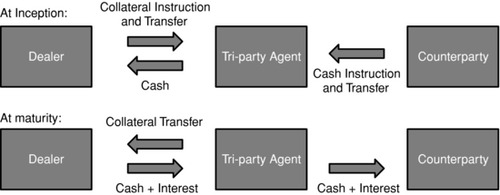
A repo transaction can be executed as a bilateral repo or tri-party repo. In a bilateral repo, the counterparty borrows cash directly against a security, which is posted as collateral or via an executing broker. In a tri-party repo, a tri-party agent—normally a custodian bank—acts on behalf of the transacting parties to carry out the transaction requirements, such as settlement, margin maintenance, and collateral substitution. A tri-party repo reduces execution risk for lenders of cash and provides borrowers of cash greater flexibility with collateral substitution. Today, tri-party repos are the most prevalent form of repo contract in the United States. According to the Payments Risk Committee, FRBNY, as of Q1 2010, the U.S. tri-party repo market was estimated to be around $1.7 trillion, down from $2.8 trillion in early 2008. It is also a highly concentrated market with the top 10 cash borrowers accounting for 85 percent of the tri-party repo. The top 10 cash lenders provided 65 percent of the funds. Bilateral repos and tri-party repos are contrasted in Exhibits 4.13 and 4.14, respectively.
Exhibit 4.13 Bi-Lateral Repo
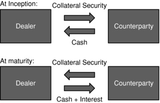
Exhibit 4.14 Tri-Party Repo
The repo is a money market instrument that plays a critical role in the efficient functioning of the bond market. It is the lifeline of modern financial markets, as it allows dealers and other market participants to access liquidity to finance their trading and risk-management activities. Underwriters of a new issue in government or corporate debt can hedge by taking an offsetting short position in an existing issue with similar risk. A liquid repo market allows the underwriter to borrow the security in the repo market and deliver against the short position. It also enables short sales by market participants. Central Banks use the repo market to add to and withdraw reserves from the banking system to manage their monetary policy. During market turbulence, central banks have used repo markets to quickly pump liquidity into the financial system and control systemic risk. Recently, policy makers at the FRBNY have been testing the reverse repo as a potential tool to unwind the bank's massive liquidity infusion program following the 2008 credit crisis.
Due to the wider selection of collaterals that can be posted against a GC repo, these repos are uniform across financial institutions for each maturity and are closely correlated to unsecured money market rates. The specified repo rate on a specific security, on the other hand, can be lower than the GC repo rate. If so, the difference represents the implicit borrowing fee for the security, and the security is said to have been “on special.” If the GC repo rate is low, then a security that has gone special can even have a negative repo rate. This allows holders of the security to earn excess return on their holdings. Negative repo rates for some securities are common during short squeezes. During a short squeeze there is heavy demand from short sellers to borrow the specified security for delivery against their short position. Negative repo rates can occur often in “on the run” government securities or “cheapest to deliver” bonds in the bond futures market.
Even though a repo is similar to secured lending it does not eliminate all credit risk. If the seller fails to fulfill his obligation at the repo's maturity to repurchase the security previously sold, the buyer may keep the security, and liquidate it to recover the cash. However, the buyer may incur a loss if, during this period, the security has lost value. To mitigate this risk repos are over collateralized (haircut), as well as subject to daily mark-to-market margining.
Since the repo market is a key provider of liquidity, its failure can cause a liquidity crisis. Gorton (2009) argued that the 2007 panic was caused by the repo market. He argues that until August 2007 the haircut on structured debt was close to zero. This went up to 45 percent by the end of 2007. The increase in haircut forced a massive deleveraging causing a panic in the market. A good barometer for the health of the repo market and its liquidity is the statistics on repo “fails” published by the FRBNY and the Libor-OIS spread. The Libor-OIS spread is the rate differential between the London Interbank Offered Rate (hereinafter LIBOR) and the overnight swap index. This unusual behavior of this spread is evident in Exhibit 4.15.
Recently, the FRBNY looked into the infrastructure supporting tri-party repo agreements. Subsequently they issued a white paper to discuss policy concerns and established a task force to address these concerns. The following issues were believed to have the potential to amplify instability in the financial system and cause severe market disruption:
- The markets’ reliance on large amounts of intra-day credit made available to cash borrowers by the clearing banks that provided the operational infrastructure for the transactions.
- The risk management practices of cash lenders and clearing banks that were inadequate and vulnerable to pro-cyclical pressure.
- Lack of effective plans by market participants for managing the tri-party collaterals of a large securities dealer in default, without creating potentially destabilizing effects on the broader financial system.
The repo market is smaller today as the financial system de-leverages and market participants adjust their investment management practices.
DERIVATIVES MARKETS
Derivatives play a key role in fixed-income portfolio management. A derivative is a financial instrument (or contract between two parties) whose value is dependent upon, or derived from, the price of one or more “underlying” financial instruments. Institutional portfolio managers use derivatives to manage the overall risk and positioning of their portfolios. Dealers of derivative products offer investors customized solutions for their hedging needs. Some derivatives are structured to be tax efficient. Issuers use derivatives to manage their funding structure or hedge their issue risk.
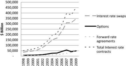
Together, the cash and derivative markets offer traders seeking alpha opportunities a sizable investment universe. Most derivatives trade over-the-counter, but financial reforms, being put in place following the credit crisis in 2008, are beginning to transform this market with the expectation of a significant expansion of exchange involvement. Dealers in derivatives markets provide products with both simple and complex cash flows that are used by both portfolio managers and risk managers. According to the Bank for International Settlements (BIS), the total notional amount of interest rate contracts outstanding has grown from $50 trillion in 1998 to $449 trillion in 2009. This is a validation of the tremendous success and importance of these products in the global capital markets. The recent growth of the fixed income derivatives markets is depicted in Exhibit 4.16.
Exhibit 4.16 OTC Interest Rate Derivative Notional Outstanding
Source: BIS Quarterly Review, June 2010.
While the landscape of derivatives can be overwhelmingly complex for many investment professionals, the plain-vanilla products can accomplish most portfolio objectives. The liquidity and transparency of such products usually more than offset the additional structural benefits of the more complex instruments. The plain vanilla products include futures, swaps, swaptions, caps, and floors.
Interest Rate and Government Bond Futures
Interest Rate and Government bond futures provide market participants with liquid, standardized exchange-traded instruments to manage their interest rate risk.
Interest Rate Futures: These are obligations that commit market participants to lend or borrow a specified notional amount at a specified interest rate on a specified future date for a specified term. Buying an interest rate futures contract is equivalent to lending the notional amount, while selling an interest rate futures contract is equivalent to borrowing the notional amount. Eurodollar futures contracts, which trade on the Chicago Mercantile Exchange (CME), Euribor futures, which trade on the Euronext, Short Sterling futures, which trade on the London International Financial Futures, and Options Exchange (LIFFE), and Euroyen futures, which trade at the Tokyo Financial Exchange (TFX) are some of the major interest rate futures contracts traded globally.
Interest rate futures are quoted as 100, less the futures interest rate expressed on an annual basis. That is, the futures price rises when the rate goes down and declines when the rate goes up. For example, the 3-month Eurodollar futures traded on the CME indicate the 3-month rate on U.S. dollars deposited in commercial banks outside the United States (Eurodollar time deposit or LIBOR rate) at the final settlement date for the contract and quoted 100 less this rate. If the price today for December 2011 Eurodollar futures contract is 99.15 then it implies that the futures LIBOR rate for 3-months beginning December 2011 is 0.85 percent. The daily price fluctuations of a futures contract reflect the market expectations for the designated interest rate on the final settlement date. During the life of the futures contract, the futures rate will be less closely related to the current cash market interest rate and more closely related to the forward rate for the final settlement date. However, as the contract approaches the final settlement date, the futures rate begins to converge to the cash market interest rate. On the final settlement date, the futures rate will be exactly the same as the cash market interest rate. This convergence is guaranteed by the fact that the final settlement price of the Eurodollar futures contract is determined by the 3-month LIBOR cash market rate on the last day of the trading.
Government Bond Futures: A government bond futures contract is an obligation to take or to deliver—depending on whether one is long or short—a specified security at a future settlement date. Settlement can be with cash or delivery of the specific security, depending on the terms of the contract. Most traders will close their position by an offsetting transaction prior to the last trading date in the contract's life. However, if a deliverable contract remains open at the expiration of a contract, then it requires physical transfer of the security. Some of the leading government bonds futures contracts are: the U.S. Treasury note and bond futures (CBOT), U.K. Gilt futures (LIFFE), Japanese JGB futures (TSE), and the German Bobl, Schatz, and Bund futures (Eurex). The contract specifications for the various interest rate and bond futures that trade on the CBOT is given in Exhibit 4.17.
Exhibit 4.17 CBOT Interest Rate and Treasury Futures Contract Specifications
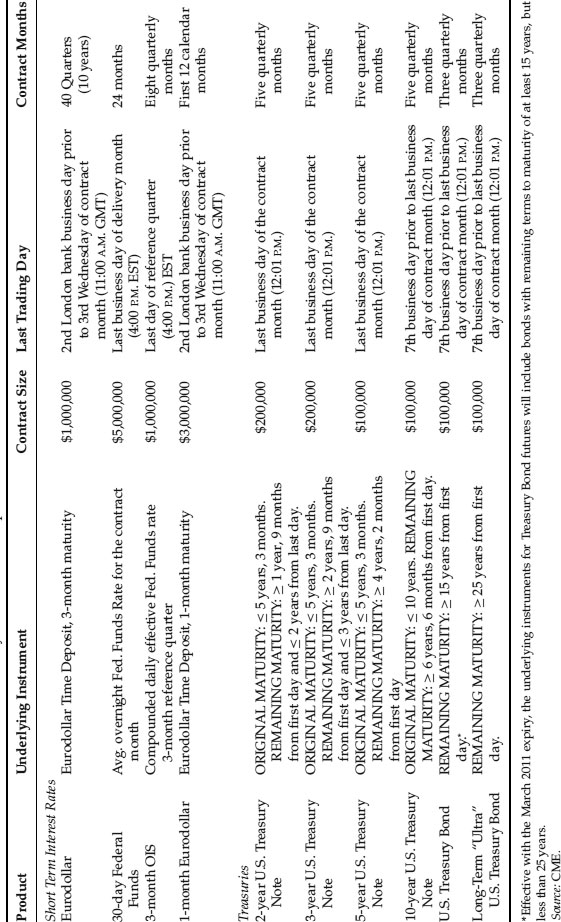
It is important to note that, due to the bond and note futures contract specifications, the buyer of a futures contract is simultaneously short several delivery options. In the case of U.S. Treasury futures, the seller of the futures contract can choose which bond to deliver (quality option), delay the delivery between the futures close and notification deadline (wildcard option), and switch the bond to be delivered between the futures close and the notice date (switch option).
Forward Rate Agreements and Interest Rate Swaps
Forward Rate Agreements (FRAs): These are contracts that pay or receive a fixed rate of interest on notional principal in exchange for receiving or paying the going Libor rate at a future point in time. The payment is made at the reset, but discounted from final maturity because the underlying cash instrument would be paid then. The market convention is to reference the purchaser of a FRA as the one paying the fixed rate. Note that, because of its structure, buying an interest rate future is equivalent to selling an FRA with the same International Monetary Market (IMM) dates.
Interest Rate Swaps: Interest rate swaps are agreements between two counterparties to exchange one stream of interest payments for another stream of interest payments. The interest payments are calculated based on a specified notional principal with typically no exchange of this notional principal. The most common interest rate swap involves the exchange of a fixed interest payment for a floating interest rate payment based on a reference rate (such as LIBOR). An interest rate swap agreement wherein the counterparty receives a fixed interest rate and pays a floating interest rate has a position equivalent to the economic risk of purchasing a bond.
There are many varieties of interest rate swaps that are considered exotic instruments. A callable swap allows one of the counterparties to cancel the swap. Effectively it is a swap with an embedded swaption. Another variant is the switchable swap. It is like the callable swap except the terms of the swap are changed rather than cancelled. For example, a counterparty can switch a floating leg to a fixed leg. The change of terms in callable swaps and switchable swaps is discretionary, whereas in the case of trigger swaps it is specified. For instance, the swap changes if the LIBOR on any roll day exceeds a specified level.
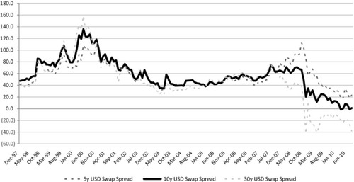
The standard LIBOR fixed-for-float interest rate swap is priced such that the present value of the fixed payment is equal to the present value of the floating rate payment. The discount rate for discounting the cash flows and the floating rate (or forward rate) is obtained from the swap yield curve. Since interest rate swaps are OTC instruments,1 it exposes the involved parties to counterparty credit risk. The absence of any exchange of principal lowers this risk. Additionally, the terms of the contract specify margining requirements that further mitigate this counterparty credit risk. Historically, USD interest rate swap rates have been quoted at a spread over Treasury yields of the same maturity. This is called a swap spread. The spread has been viewed as a reflection of the credit risk premium on the banking system. However, swap spreads are not the same across currencies. Therefore the idea that swap spreads reflect the banking credit risk has been a less than satisfactory explanation. Much has been debated and written about the rationale for USD swap spreads to be wider than EUR swap spreads when the same financial institutions dominate both these markets. The difference has been explained based on technical factors and differences in the financing activities of the corporate sector in the US and Europe. If there is one fact that has been accepted uniformly, it is that the swap spread would be positive. The collapse of Long-Term Capital Management in 1998 was a painful lesson for some on the dangers of hedging interest rate risk by shorting Treasuries. The hedging strategy failed in 1998 as a flight to quality resulted in Treasuries rallying while the swap spread widened. As a result, there has been a migration from Treasuries to interest rate swaps for hedging interest rate risk.
However, after the September 2008 bankruptcy of Lehman, the market behavior of the swap spread changed significantly. The USD 5-year, 10-year, and 30-year swap spreads reacted very differently in the months after the bankruptcy of Lehman, and they now trade at very different levels. The five-year swap spread widened and subsequently declined. The 10-year and 30-year swap spreads, instead of widening, declined, and have traded down. In August 2008 the 5-year, 10-year, and 30-year swap spreads were around 93bps, 68bps, and 40bps, respectively. At the end of August 2010 these were at 23bps, 1bps, and -38bps. These low, even unthinkable, negative swap spreads for the 30-year, were initially viewed as a short-term phenomenon driven by technical factors, such as the unwinding of relative value trades, and other duration hedging activities by institutional investors. But, as of the time of this writing, this condition has not changed and it is unclear if it will continue. The August 2010 swap spreads are depicted in Exhibit 4.18.
Options
Interest Rates Futures Options: These are exchange-traded options on interest rate futures contracts (e.g., Eurodollar futures). A call option gives its holder the right, but not the obligation, to buy the underlying futures contract while the put option gives its holder the right, but not the obligation, to sell the underlying futures contract. An American-style contract allows the exercise of the option at any time on or before the expiration date, whereas a European-style contract can only be exercised on the expiration date. The buyer of a call option in effect has the right to establish a long position in the underlying futures contract, while the buyer of a put option has the right to establish a short position in the underlying futures contract. The price at which the option holder can exercise his option to buy or sell is referred to as the strike price. Since the futures price moves inversely with the interest rate, the purchaser of a call option will profit when the interest rate declines further than the rate implied by the strike price. Similarly, a holder of a put option will gain when the interest rate rises more than the rate implied by the strike price. Options can be traded on the Eurodollar, the Euribor, the Euroyen, and short Sterling futures contracts. Generally these options are American-style.
Bond Futures Options: Similar to interest rate futures options, the bond futures options are exchange-traded options on government bond futures contracts. The option can be a call or a put option and are generally American-style.
Caps and Floors: A caplet is a call option on an FRA, that is the right to pay fixed at the expiration date. A floorlet is a put option on an FRA. Caps and floors are collections of consecutive caplets/floorlets with each caplet/floorlet being independently exercisable. A long cap position pays out when the rate is above the cap rate. This is similar to a put option on a bond. Similarly, a long position in a floor pays out when the rate is below the floor rate, which is similar to a call option on a bond.
Swaptions: The European swaption is the right to enter into an interest rate swap at an agreed-upon fixed interest rate on the expiration date of the contract. The right to pay a fixed interest rate is called a payer swaption, and the right to receive a fixed interest rate is called a receiver swaption. It is important to distinguish caps and floors from swaptions. Caps and floors are portfolios of options on FRAs, while swaptions are options on portfolios of FRAs.
The derivatives markets are undergoing dramatic changes as market participants and regulators globally respond with reforms. The traditionally over-the-counter derivative market is moving to exchanges. Under the Dodd-Frank Wall Street Reform and Consumer Protection Act passed by U.S. lawmakers, plain-vanilla swaps must be cleared through a registered clearinghouse and executed on a registered trading platform, that is, exchanges. Only non-financial entities will be exempt from clearing requirements, provided that they are not “major swap participants,” use the swaps to hedge commercial risks, and are able to meet their financial obligations. The swaps include commodity, credit, currency, equity, interest rate, and foreign exchange swaps. The margin and capital requirements for major swap participants will be set higher by the regulators. Additionally, there will be more extensive reporting requirements on swap activities. This is a significant change for the derivative market that has caused considerable anxiety as the market awaits more clarity. The silver lining in all this is that it will bring much-needed transparency and stability to the derivatives markets. The benefits of derivative products include the ability to effectively hedge portfolio risks, manage asset-liability risks, and reposition portfolios efficiently. The derivatives markets are, and undoubtedly will continue to be, an integral part of investing, hedging, and debt issuance for financial and non-financial entities alike.
PRICE–YIELD RELATIONSHIP
The relationship between a bond's price and its yield is nonlinear and can further vary depending on the terms of the security. For a bond with no embedded option this can be expressed as follows:
![]()
where C is the coupon, α (ti - 1 ,ti) is the accrual factor between time ti and ti–1, y is the bond's yield, Par is the principal, and tN is the maturity in years. Macaulay (1938) proposed duration as a measure for the price volatility of a bond investment. (Note that the price equation above and the Macaulay duration equation below are both assuming that there is only one coupon payment per year.)
Macaulay's Duration measures the average life of a bond investment where the weight is the present value of each cash flow divided by the price of the bond. The concept of duration has since been modified and interpreted as price sensitivity of a bond to a change in its yield. Below is the relationship between Modified Duration and Macaulay's Duration. (Note: frequency refers to the number of coupon payments per year. If the bond paid semiannually, for example, the frequency would be 2.)
![]()
Market convention uses the term “duration” to refer to modified duration. Mathematically, duration is the linear approximation or the first-order effects of the price yield curve. Higher coupon bonds have a lower duration compared to lower coupon bonds for the same maturity. Longer maturity bonds have a higher duration than shorter maturity bonds. Another important bond attribute is “Convexity.” It is the change in duration as the yield changes. Convexity is the quadratic term or the second-order effects of the price-yield relationship. Convexity captures the curvature of the price-yield curve. The relationship between the change in the price of a bond, P, and a change in its yield, y, can be approximated by the first and second terms of a Taylor series expansion.
![]()
For a small change in yield we can ignore the error term and rewrite the above expression as follows:
![]()
For a bond with no embedded options, the bond's price is negatively related to its yield and has positive convexity. Positive convexity means that for a given change in yield, a bond's price increases more when the yield declines than when the yield rises. Coupon, maturity, call, put, and sinking fund features can change the degree of convexity, and change it from positive to negative. Bonds that are callable will display negative convexity in some regions, since the call option limits price appreciation when yields decline. The duration and dispersion of cash flow determines the level of convexity. The convexity of a non-callable bond is proportional to the square of its duration, and it is higher when the dispersion of cash flow is higher. Therefore, long-term bonds are more convex than short-term bonds. Among a portfolio of bonds with the same duration, the zero-coupon bond will have the least convexity since it has no cash flow dispersion. Positive convexity is a desirable property since it can enhance returns. This bias is reflected in market prices, and its value depends on yield volatility. Understanding both duration and convexity is important in bond portfolio management. For example, a barbell portfolio of short-term and long-term zero-coupon bonds with more dispersed cash flow has more convexity than a similar duration, intermediate term, zero-coupon bond.
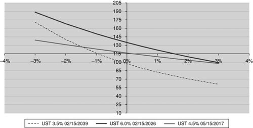
The price-yield curves for several U.S. Treasury bonds with different coupon rates and maturity are depicted in Exhibit 4.19. As the yield declines, the UST 3.5% 2/15/2039, the lowest coupon bond, begins to increase more rapidly than the others. On the other hand, as yield increases, the lowest coupon-paying bond's price declines more than the price of the higher coupon-paying bond.
Exhibit 4.19 Bond Price versus Yield
Not all bonds have fixed interest cash flows with a bullet maturity. The terms of a bond can include floating rate payments, step-up or step-down coupon payments, sinking fund and amortization schedules, call provisions (callable), or put provisions (putable). Duration and convexity can be difficult to calculate analytically, given the possibility of a variety of bond payment terms and embedded options. Moreover, the analytical calculation is accurate only for a small change in yield and not practical for a large portfolio of bonds. Therefore, in practice, duration and convexity are estimated numerically by changing the yields and repricing the bonds. This process then allows for inclusion of the effects of non–plain vanilla features, such as optionality. The resultant measures are called effective duration and effective convexity.
Exhibit 4.20 Duration and Convexity for a Sample of U.S. Treasuries
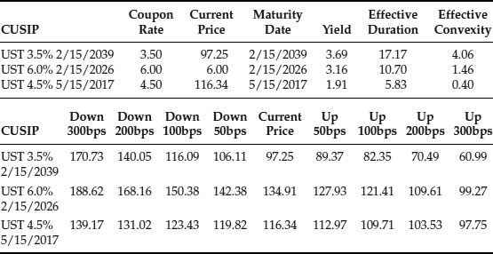
where P(y0) is the current price at yield y0, P(y+) is the bond price when yield increases to y+ and P(y−) is the bond price when yield decreases to y−. This is simply a numerical method to estimate first- and second-order derivatives (in the mathematical sense of a derivative). Exhibit 4.20 below shows the effective duration, the effective convexity, and the change in price for various changes in yield for a portfolio of U.S. Treasury bonds. The duration of the UST 3.5% 2/15/2039 bond is 17.17, meaning that for a 100bps change in yield the price will change by 17.17 percent. Its convexity is 4.03, which implies that for a 100bps change in yield the convexity will add another 2.01 percent price change.
The duration and convexity of a portfolio can be estimated by using the change in value of the entire portfolio. For a small change, in yield the estimated price change, using duration and convexity as the basis for the estimate, will be close to the actual change. However, as the change in yield gets larger, the estimation error can increase considerably.
Duration and convexity are useful tools for government bond futures trading. Government bond futures generally permit the delivery of bonds within a range of maturities. This is known as the deliverable basket. For example, the 10-year U.S. Treasury bond futures permit delivery of coupon-bearing U.S. Treasuries with remaining term to maturity of at least 6.5 to 10 years from the first day of the delivery month. Since many bonds are available for delivery, the exchange homogenizes it with the use of a fixed conversion factor. The conversion factor for the 10-year U.S. Treasury bond is determined so that if every bond eligible for delivery yielded 6 percent, then there would be no preference for delivering any particular bond. The invoice price for the futures contract at the last settlement date is the futures settlement price, times a conversion factor, plus accrued interest. Since it is unlikely that all bonds in the market yield 6 percent, the further the market is away from 6 percent the less effective the homogenization becomes. The bond that is cheapest to deliver, known as the CTD bond, has the lowest basis. Basis is the price of a deliverable bond less the futures invoice price. Net basis is basis less carry, where carry is the bond coupon plus accrued interest, less the funding cost. The funding cost is determined by the repo rate. The duration and convexity of each bond in the basket is important in determining which deliverable bond could become the cheapest to deliver under different rate scenarios. This is the key to understanding a complex and highly sophisticated form of fixed income trading known as basis trading.
Exhibit 4.21 U.S. Treasury Bond Price Yield Normalized by Conversion Factor
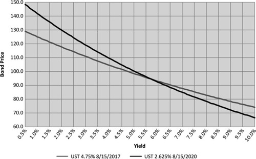
Exhibit 4.21 shows the price changes for two deliverable bonds normalized by their respective conversion factors. When the yield declines, the low-duration bond becomes more attractive to deliver. High-duration bonds are attractive to deliver when yields rise. The shape of the yield curve (to be discussed later) will also affect the relative cheapness. If the yield curve steepens as yield falls, then, this will offset some of the incentive to deliver the low-duration bond. Similarly, if the yield curve flattens as yield rises, the incentive to deliver high-duration bonds will be somewhat offset. If the yield curve is inverted, then shorter-maturity bonds will be cheaper to deliver.
THE YIELD CURVE
Term Structure
The term structure of interest rates, commonly referred to as the “yield curve,” describes the relationship between the market yield and maturity for securities with a similar credit risk. Typically, the yield curve is upward-sloping. That is, long-term rates are higher than short-term rates. The upward-sloping yield curve has been rationalized based on several plausible explanations including (1) a liquidity risk premium for investing longer term, (2) a term risk premium for higher volatility assets, and (3) inflationary expectations. An inverted yield curve has generally been viewed as a precursor of recession.
The yield curve plays a central role in the valuation, trading, and risk management of fixed income portfolios. The yield curve has embedded in it the consensus market views on the economy, inflation expectation, risk premia, and demand/supply imbalances. Several trading strategies and portfolio actions are driven by views on the current and future shape of the yield curve. The yield curve is essential to the valuation and hedging of fixed income assets. Since a fixed income portfolio pays out a stream of cash flows, a more appropriate gauge of its interest rate sensitivity is the “Key Rate Duration.” The key rate duration for a bond is the price sensitivity of the bond to different points on the yield curve. This is done by changing the rates at different points along the yield curve and repricing the bond. Embedded in the yield curve is the market's implied forward rate curve, which is the short-term rate at various forward dates. Trading in futures and interest rate swaps is motivated by a trader's views on the implied forward curve.
Exhibit 4.22 Benchmark Government Bond Yield Curve, August 16, 2010
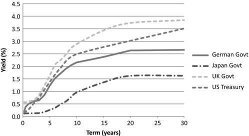
Exhibit 4.22 depicts the yield curves for the United States, the European Union, the United Kingdom, and Japan based on benchmark government bonds. The money market deposit and LIBOR swap rates for USD, EUR, JPY, and GBP are shown in Exhibit 4.23. These quoted market rates are only indicative of the interest rate term structure and not applicable for many trading decisions and valuations. More precise and accurate information on the yield curve is needed. This is done by building the discount curve, par curve, zero-coupon curve, and forward rate curve from the quoted market rates. The discount curve indicates the discount rate for discounting cash flow at future dates, while the par curve represents the yields on bonds issued at par at different maturity dates. The zero-coupon curve, also known as the spot rate curve, represents the yields on zero coupon bonds for different maturity dates. The forward rate curve shows the implied forward rates for specific terms at different dates in the future. These curves are related to one another and can be viewed as just alternate representation of the same information. It is also important to note that the expected interest rates implied by these curves (particularly the forward curve) are unique in that they are the prevailing rate currently offered by the market and can be locked-in. This can be done with a FRA or with an interest rate futures contract. In the LIBOR swap market, the method used to construct the yield curve is called bootstrapping the yield curve, and in the government bond market it is called the fitted yield curve.
Exhibit 4.23 Deposit and Swap Rates, August 16, 2010

Bootstrapping the Yield Curve
Bootstrapping the yield curve (also called zero coupon stripping) refers to a process whereby each data point along the yield curve is generated progressively, so that it is consistent with the market interest rates used as inputs. The LIBOR swap curve is built by splicing together rates from multiple markets and instruments. The selection of markets and instruments depends on the purpose and currency, but it is generally built using a combination of money market deposit rates, interest rate futures prices, and swap rates. Since the objective of building the yield curve is to derive the term structure of interest rates for trading, hedging, and valuation purposes, a prudent rule to follow is to use the rates and prices that are the most liquid and actively traded in the market as input quotes. It is common to use money market deposit rates from overnight to the first few weeks or months, followed by interest rate futures for several quarters, depending on market liquidity, and, finally, the swap rate.
The extraction of the discount factor from the deposit rate is the most straightforward, due to the simplicity of the money market instrument.
![]()
where t0 is the current date, Z(t0, t1) is the discount factor for time t1, r(t1) is the deposit rate for time t1, and α(t0, t1) is the interest-accrual factor based on the day count convention for the interest rate.
The relationship between discount rate and forward rate can be summarized as follows:
![]()
where f(t1,t2) is the forward rate between time t1 and t2. If the discount factor to time t1 is known, and the forward rate between time t1 and t2 is known, then the discount factor for time t2 can be calculated. The forward rate can be calculated from the futures prices. If, as a quick approximation, the forward rate can be assumed to be equal to the futures rate, then it is simply 100 less the futures price. However, if one would like to be more precise, then the futures rate needs to be adjusted for convexity bias to derive the forward rate. Convexity bias arises since the futures contract is settled daily and is linear with respect to the interest rate whereas a FRA is non-linear with respect to the interest rate (due to the discounting mechanism) and settled at maturity. Due to this difference in the settlement procedure, there is an advantage to consistently short the FRA and hedge it with a short futures contract. This is recognized by the market and reflected in the market prices of the futures contract. The convexity bias is small for near-dated futures contracts but can be larger for far-dated contracts. The convexity bias will result in the futures rate being adjusted downwards, and depends on the volatility of the forward rate, and the correlation between the forward rate and the zero-coupon bond price at the maturity of the forward rate. Each discount factor can be progressively calculated with the help of the above expression until all futures prices have been used.
The par swap rate, S(t0, tn), for time tn, can be linked to the discount factors as below:
![]()
Alternatively,
![]()
If all the discount factors up to time tn–1 are known then, using the swap rate for time tn, we can determine the discount factor for Z(t0,tn) for time tn.
Since the market may not trade all points on the yield curve, any deposit rate or swap rate that is needed for building the curve, but not quoted, must be interpolated from the other quoted market rates. The interpolation techniques used to stitch the curve between deposit rates and futures rates and determining any unknown swap rates is important, so as to obtain a smooth yield curve or smooth forward curve.
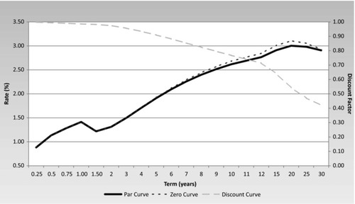
With the discount curve, it is now possible to calculate the zero-coupon curve, forward curve, and par curve. The discount curve can be directly used in discounted cash flow models to value other financial instruments. Examples are depicted in Exhibit 4.24.
Exhibit 4.24 USD Par, Zero-Coupon, and Discount Curves, September 3, 2010
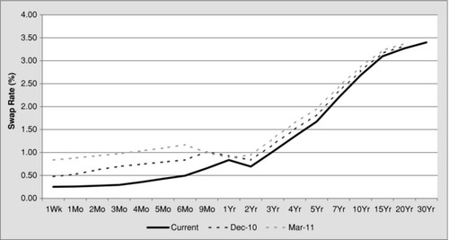
Perhaps the most important perspective on the market can be obtained by looking at the forward curve. The forward curve shows the evolution of the yield curve as implied by the current market yield curve. Exhibit 4.25 depicts the current versus implied forward curve for USD for December 2010 and March 2011. This indicates that the market is expecting short-term rates to rise by around 60bps and the yield curve to flatten slightly. If a trader believes that the rates will increase significantly more, or if he expects the curve to flatten more significantly, then he can execute transactions in the cash and/or derivative market to monetize the view.
Exhibit 4.25 USD Forward Curve, September 3, 2010
Fitted Yield Curve
The bond market trades a wide range of bonds that differ in their coupons, payment dates, and maturities. Unlike the swap market, which quotes uniform rates for any specific term, the prices of bonds for any maturity can differ widely due to differences in liquidity, coupon, and other factors. Therefore, in the bond market, a fitting algorithm is needed to construct a yield curve. The motivation for bootstrapping the yield curve in the swap market was driven by the need to gain an insight into the market's implied expectations and for the valuation of many OTC products. The objective of the fitted yield curve in the bond market is for time series analysis of the yield curve and rich/cheap analysis of the bonds for relative-value trading strategies. The fitting algorithm is useful in identifying bonds that are significant outliers compared to historical norms. A bootstrapping algorithm guaranteeing that the constructed yield will recover the bond prices is not desirable if there is recognition that technical factors in the market can distort some bond prices. The objective is to apply a consistent methodology to identify the outliers for trading purposes.
The fitting algorithm for bond yield curves can be distinguished by those that fit the bond yields and those that fit the market prices. The models that fit the yield specify a functional form for the yield curve and use a least squares method to estimate the coefficient of the function that can best fit the bond yield used in the sample. The methodology, with a suitable function, can produce a smooth yield curve but can still be theoretically unsound. The biggest objection to this approach is that it does not require that cash flows occurring at the same date be discounted at the same rate. The price-fitting model begins by specifying a functional form for the discount factor function, and uses the bond prices in the sample to estimate the coefficient of the function. Further, constraints that the discount factor be one at time zero, and be downward sloping with respect to time, can be explicitly incorporated.
A simple function that works well for this purpose is to model the discount curve as a linear combination of m basis functions where each basis function is an exponential function. In this approach, the discount factor at time tn is
![]()
where ak and b are the unknown coefficients to be estimated. Since the discount factor is one at time zero the following constraint can be derived:
![]()
A reasonably good fitting yield curve can be obtained with five basis functions. The procedure to estimate the coefficients for a sample of bonds can be done with ordinary least-squares regression.
INTEREST RATE MODELS
Interest rate models are important for managing interest rate risk and for the valuation of securities. Interest rate modeling can be viewed from two different perspectives depending on the market. Fixed income cash bond portfolio managers have an interest in the statistical modeling of the time series properties of interest rates for predictive purposes. Volatility and correlation are estimated using observed market data. Often, techniques such as principal component analysis are used to explain the movements in the yield curve. In the interest rate derivatives market, on the other hand, the preferred approach to modeling interest rates is to derive it from market prices. Volatility and correlation are implied from the prices of liquid plain-vanilla derivative products.
Black-Scholes (1973) pioneered the approach to pricing derivative securities. If the terminal payoffs of a derivative security can be perfectly replicated then, under no-arbitrage conditions, the value of the derivative security should be the same as the value of the replicating strategy. This was the main principle behind their pricing equation for an equity call option. Their model assumed that the underlying stock price follows a lognormal distribution. The Black-Scholes intuition of perfect replication continues to be the fundamental principle behind the design and valuation of derivative securities in the market. Another perspective on the Black-Scholes approach is the principle of “risk-neutral” valuation. Since a derivative instrument's payoff can be perfectly replicated, it is valid to assume a market that is risk-neutral, that is, indifferent to individual risk preferences. The value of a derivative instrument, therefore, is the present value of the expected payoffs where the expected payoffs are determined according to the risk-neutral distribution and discounted by the risk-free rate. A few years after the Black-Scholes seminal paper was published, Black (1976) presented a modified approach to price options on futures. This model assumes that futures prices are lognormally distributed. This model has been used by the market to value options on interest rate futures, options on bond futures, caps, floors, and swaptions. From a strictly theoretical perspective, the use of the Black (1976) model to price all these instruments is inconsistent. A lognormal forward rate is not consistent with a lognormal swap rate. Likewise, a lognormal bond price is not consistent with a lognormal swap rate. The market is fully aware of these inconsistencies and reflects them in the volatilities used to price these instruments using the Black model. Therefore, in the plain vanilla interest rate derivative markets, the model simply acts as a way to translate price into implied volatilities.
Options embedded in bonds or in derivative securities with a more complex payoff cannot always be priced with the Black model. A more explicit model for the evolution of interest rates is needed to price these securities. These interest rate models follow the basic principle of the Black-Scholes model, namely, a no-arbitrage principle. However, they also bring other elements unique to interest rates, such as mean reversion. The early models for interest rate derivatives were called the short-rate models. These models began with an assumption of a stochastic process for instantaneous short rates. The models are designed to be consistent with today's term structure of interest rates. Hence they are also called no-arbitrage models. Ho and Lee (1986), Hull, and White (1990), Black, Derman and Toy (1990), and Black and Karasinski (1991) are some examples of short-rate models. The consistency of these models to the options market is achieved by calibrating the model. The models are used to price calibrating instruments (generally plain-vanilla swaptions or caps and floors) and parameters estimated so it can best fit the price of the calibrating instruments.
The next-generation models moved away from modeling the short rate and switched to modeling the entire term structure of interest rates. An early pioneer of this approach was the model by Heath, Jarrow, and Morton (1992) (HJM). They proposed a model for the evolution of a continuum of forward rates. The volatilities of the forward rates and correlations between them are left as exogenous inputs. The covariance function and the initial yield curve are the only inputs. The problem with HJM is that a continuum of instantaneous forward rates does not exist. The market is liquid only in certain instruments and at certain maturities. HJM does not have a satisfactory analytical solution and the numerical simulation can be computationally demanding. The Brace, Gatarek, and Musiela (1997) (BGM) model is a practical, discrete-time implementation of an HJM-type model. The BGM model considers a set of consecutive forward LIBOR rates and assumes that they follow a log-normal distribution. Since the assumption of log-normal forward rates is in keeping with the market convention of using the Black model to price vanilla options, market volatility can be employed directly as an input into the model.
Interest rate derivative models are complex, therefore their calibration is an essential part of model development. It is critical to understand the objective of calibration. Since the model is used not only for valuation but also for hedging, it is necessary that the model not only recover the market price, but that it is also able to track the evolution of volatility and correlation in the market.
Trading Strategies
The breadth and depth of fixed income markets offers investors opportunities to implement a variety of strategies to exploit their views and observations on the market. Two common strategies are government bond basis trading and curve trading.
Government Bond Basis Trading: Basis trading is the buying (selling) of government bonds and the simultaneous selling (buying) of government bond futures. A trade that involves buying the government bond in the cash market and selling the bond futures contract is referred to as “going long the basis.” The opposite strategy is referred to as “going short the basis.” When the basis is tight, long basis trades can be profitable. When the basis is wide, short basis trades can be profitable. It is unusual to have a negative basis. If the basis were to become negative, a trader could realize arbitrage profits by buying the cash bond and delivering it against the futures contract. The risk and return of such a trade is generally very low and requires a lot of capital.
A trader would normally employ a lot of leverage to improve the return on capital from such trades. Changes in repo rate, yield curve, and supply factors are important determinants of basis. Another key determinant for changes in basis is the conversion factor used by exchanges to adjust the futures invoice price for each bond in the deliverable basket. The futures invoice price of any two deliverable bonds always moves at a fixed ratio based on the conversion factor; it does not change as the bond prices changes. As the market moves away from par, the conversion factor begins to disproportionately affect the basis of each bond. When the price rises, the price of the high coupon (low duration) bond will change less than the low coupon (high duration) bond with the same maturity. The reverse is true when the bond price declines. Since the conversion factor does not change, this cheapens the high coupon/low duration bonds in a rally. During a sell-off, the low coupon/high duration bonds become cheaper. Basis trading is not without risks. Due to the high leverage employed by the strategy, it is subject to significant risk if the repo counterparty fails to deliver.
Curve Trading: The U.S. bond markets offer many kinds of inter- and intra-market spread-trading opportunities. The on-the-run versus off-the-run spreads involve trading the benchmark bond against an older bond with similar maturity. In the case of a swap spread trade, a bond is traded against a swap. In contrast, curve trading involves trading the slope and the shape of the yield curve.
Exhibit 4.26 The 10-year and 2-year U.S. Treasury spreads: September 1980–July 2010
Used with permission of Bloomberg Finance L.P.
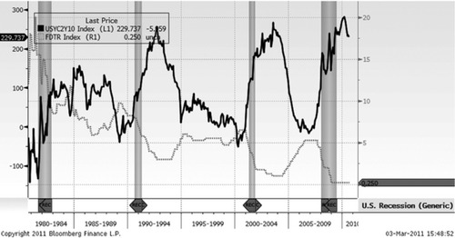
The classic trade is the curve steepener or curve flattener. Exhibit 4.26 depicts the 10-year and 2-year U.S. Treasury bond spread along with a recession indicator. Historically, the slope of the curve has been a function of the strength of the economy and Fed actions. Policy rate cuts by the Fed have been accompanied by a steepening of the yield curve while rate hikes have been accompanied by a flattening of the yield curve. A curve steepener involves shorting a longer-dated bond against a shorter-dated bond. (That is, you go short on the long-maturity bond and long the short-maturity bond.) The weights of the long position and short position are selected so as to be duration-neutral, but the position may have convexity risk. Another type of curve trade is based on views about the curvature of the yield curve. This involves going long on both a short-maturity bond and a long-maturity bond, while simultaneously going short on an intermediate-maturity bond. This is called a butterfly strategy. The weight on the bonds can be adjusted to be duration-neutral or dollar-neutral.
Consider, for example, the spread between the yields on the 5-year and 30-year U.S. Treasuries. (These are depicted in Exhibit 4.27.) The spread that was close to flat in December 2006 is at 230bps in September 2009. If a trader believes that the curve will flatten, he can sell the 5-year bond and buy the 30-year bond. The trade can be done so the dollar value of the bond sold is equal to the dollar value of the bond purchased. However, this is not a risk-neutral trade. The trader is exposed to the risk of a parallel shift in the yield curve while he is waiting for the curve to flatten. To avoid this risk, the relative sizes of the positions should be adjusted in such a fashion that the net position is duration-neutral. In Exhibit 4.28, a duration-neutral transaction is depicted together with the expected profit or loss if the yield curve steepens or flattens.
Exhibit 4.27 30-year and 5-year U.S. Treasury Yield and Spreads: December 2006–August 2010
Source: Bloomberg Finance L.P.
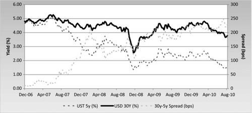
Exhibit 4.28 30-year, 5-year U.S. Treasury spread trade
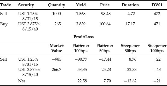
Note
1. This is beginning to change with a push by regulators to move more derivatives trading to exchanges.
REFERENCES
Black, F. 1976. “The Pricing of Commodity Contracts,” Journal of Financial Economics 3 (March): 167–79.
Black, F., E. Derman, and W. Toy. 1990. “A One-Factor Model of Interest Rates and Its Application to Treasury Bond Options.” Financial Analysts Journal (January/February): 33–39.
Black, F., and P. Karasinski. 1991. “Bond and Option Pricing When Short Rates Are Lognormal,” Financial Analysts Journal (July/August): 52–59.
Black, F., and M. Scholes. 1973. “The Pricing of Options and Corporate Liabilities.” Journal of Political Economy 81 (May/June): 637–59.
Brace, A., D. Gatarek, and M. Musiela. 1997. “The Market Model of Interest Rate Dynamics.” Mathematical Finance 7:2, 127–55.
Gorton, G. 2009. “Information, Liquidity, and the (Ongoing) Panic of 2007.” American Economic Review Papers and Proceedings.
Heath, D., R. Jarrow, and A. Morton. 1990. “Bond Pricing and the Term Structure of Interest Rates: A Discrete Time Approximation.” Journal of Financial and Quantitative Analysis 25:4, 419–40.
Heath, D., R. Jarrow, and A. Morton. 1992. “Bond Pricing and the Term Structure of the Interest Rates: A New Methodology.” Econometrica 60:1, 77–105.
Ho, T. S. Y., and S.-B. Lee. 1986. “Term Structure Movements and Pricing Interest Rate Contingent Claims.” Journal of Finance 41 (December): 1011–29.
Hull, J., and A. White. 1990. “Pricing interest-rate derivative securities.” The Review of Financial Studies 3:4, 573–592.
Hull, J., and A. White. 1993. “Bond Option Pricing Based on a Model for the Evolution of Bond Prices.” Advances in Futures and Options Research 6: 1–13.
Hull, J., and A. White. 1993. “One-Factor Interest Rate Models and the Valuation of Interest Rate Derivative Securities.” Journal of Financial and Quantitative Analysis 28 (June): 235–54.
Hull, J., and A. White. 1994. “Numerical Procedures for Implementing Term Structure Models I: Single-Factor Models.” Journal of Derivatives 2:1, 7–16.
Hull, J., and A. White. 2000. “Forward Rate Volatilities, Swap Rate Volatilities, and the Implementation of the LIBOR Market Model.” Journal of Fixed Income 10:2, 46–62.
Jamshidian, F. 1977. “LIBOR and Swap Market Models and Measures.” Finance and Stochastics 1:4, 293–330.
Jamshidian, F. 1989. “An Exact Bond Option Pricing Formula.” Journal of Finance 44 (March): 205–9.
Macaulay, F. 1938. “Some Theoretical Problems Suggested by the Movements of Interest Rates, Bond Yields, and Stock Prices in the US since 1856.” National Bureau of Economic Research.
Rebonato, R. 1996. Interest Rate Option Models. Chichester, UK: John Wiley & Sons.
Rebonato, R. 2004. Volatility and Correlations: The Perfect Hedger and the Fox. Chichester, UK: John Wiley & Sons.
ABOUT THE AUTHOR
Peruvemba Satish is managing director and chief risk officer (CRO) of Allstate Investments, LLC. He has held senior leadership responsibilities in the areas of risk management, portfolio management, and quantitative research for the past 15 years. Prior to joining Allstate, Satish was the CRO of Jamison Capital Partners. Earlier, he was a partner and the CRO of DKR Capital Partners LP. From 2001 to 2004 Satish was director of risk management at Soros Fund Management. Satish received his MA (Honors) in Economics from SUNY Binghamton in 1990 and a PhD in Finance from the University of Texas at Austin in 1994. He holds degrees in Mechanical Engineering and Economics from BITS, Pilani, India. Satish is also a CFA charter holder.