
Chapter 28
The No-Arbitrage Condition in Financial Engineering: Its Use and Misuse
INTRODUCTION
Valuation techniques used in financial engineering typically incorporate two fundamental assumptions regarding investor behavior. The first is that investors prefer more wealth to less, and will take actions to maximize future wealth. The second is that investors have an aversion to risk, which leads them to make trade-offs between expected future wealth and uncertainty (or risk) concerning future wealth.
The “preference of more to less” assumption is analytically quite tractable. Intuitively, it seems reasonable as a broad generalization, and the notion of wealth maximization can be well defined quantitatively. In contrast, the risk aversion assumption is much less tractable. It is somewhat less appealing as a broad generalization, but, more significantly, the notion of risk aversion can neither be defined unambiguously nor measured in a straightforward manner. As a consequence, valuation techniques that are able to rely solely on the first assumption have proven to be much more effective in practice than techniques that must also rely on the second assumption.
However, as powerful as these valuation approaches have proven to be in practice, there are certain limitations to their effectiveness that tend to magnify in times of market dislocation. In addition to the investor behavior assumption, these approaches also require a range of other conditions that are associated with the efficient functioning of markets, including market completeness and the perfect capital markets assumptions. The good news is that in normal markets the valuation models have proven to be quite robust and behave as if these market conditions were always to hold (even if they don't actually hold in the strict sense). The bad news is that this robustness can lead to a false sense of security, and when markets move beyond a certain tolerance, the models can fail spectacularly. In times of these dislocations many of the critical assumptions, which are often forgotten, are no longer appropriate, rendering the conclusions of the models invalid.
This chapter provides an overview of a valuation framework within which the “preference of more to less” assumption can be quantitatively expressed as an optimization problem. The necessary conditions under which this single behavioral assumption is sufficient for pricing purposes are developed and illustrated with a number of examples. In addition, the chapter explores the impact on the valuation approach in the cases when the sufficient conditions do not hold, with focus on the key assumptions of frictionless and complete markets.
THE OPTIMIZATION FORMULATION
The behavioral assumption that investors prefer more to less guides the actions of arbitrageurs who seek to construct a position of holdings that produce the possibility of riskless value for zero net investment. Arbitrage profits are typically classified on the basis of two basic types, defined as first-order and second-order arbitrage.
First-order arbitrage occurs when a portfolio can be constructed that yields positive value today with no future obligations in any state of the world. Second-order arbitrage occurs when a costless portfolio can be constructed that also guarantees no future obligations but, additionally, where there is some possibility of a strictly positive value in at least one future state.
We assume a model of a market where there are n independent securities and s possible future states at time t. Each possible future state, j, at time t has a strictly positive probability of occurrence, pjt. The vector Pt represents an s × 1 vector of time t state probabilities. The n × s matrix Mt represents security values where mijt is the value of security i in state j at time t. Note that while the distribution of values across states for a given security can be described by various measures of dispersion, including variance, the distribution itself need not be constrained to be normal. Likewise, while the joint distribution of values across states for two securities can be described by various measures of co-dependence, including correlation, joint normality need not be assumed.
The market price that investors must pay for security i is equal to qi; Q represents the n × 1 vector of security prices. An investor can purchase a portfolio with holdings of security i in the amount of xi. It is also assumed that there are no long or short constraints on the purchases of any of these securities. Thus, X, the n × 1 vector of security holdings, is unconstrained. The behavior of arbitrageurs who act to maximize first-order arbitrage can be modeled as the following multistate, single-period linear program:
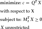
where 0 represents an m × 1 vector of zeros. This formulation follows the multistate, single-period, discrete model developed by Ross (1976).
In this formulation, an investor's objective to maximize arbitrage profits is re-expressed as an objective to minimize the cost, c, of purchasing a portfolio. The state constraints restrict the feasible solutions to those for which the net value over all trades is nonnegative for each state. Investors are able to buy (xi > 0) or sell (xi < 0) in unrestricted quantities. Given that all investors observe the same value matrix, Mt (i.e., no differential taxation or other investor-specific transaction costs), and that there are no long and short constraints, the market is assumed then to be frictionless.
POSSIBLE SOLUTIONS
Because the no-trade solution (X = 0) is always feasible, the cost of the optimal portfolio solving the minimization problem will always be nonpositive. However, while a solution to the problem is always feasible, it may be either bounded or unbounded.
There are three distinct possibilities to consider. In the first case, the problem is unbounded because the solution to the objective function (the cost of the portfolio) is negative infinity for a given set of security prices. This is the case of first-order arbitrage, whereby value may be extracted today with no future obligations, and can be scaled up in an unlimited manner. In the second and third cases the problem is bounded, as the solution to the objective function is equal to zero and, thus, no value can be extracted today.
In the second case at least one of the constraints is solved as a strict inequality. This is the case of second-order arbitrage where, given a zero initial net investment, there is some possibility of a strictly positive future value. In the third case, all constraints are solved as strict equalities. This solution is known as the no-arbitrage condition, since no first- or second-order arbitrage opportunities are available for a given set of security prices.
MARKET EQUILIBRIUM
In this general model, the preference of more to less is the sole assumption that guides investor behavior and, as a result, governs the equilibrium pricing of securities in markets that are frictionless and efficient. The actions of arbitrageurs as they attempt to maximize arbitrage profits therefore serve to force prices of relatively underpriced securities higher, and those of relatively overpriced securities lower, until all first- and second-order arbitrage opportunities have been eliminated.
As a result of these market dynamics, we can then assume that the security prices observable to the general investor (post the actions of arbitrageurs operating at the margin), are governed strictly by the no-arbitrage condition. This is the key conclusion of the model, and is reflected by the familiar expression, “the Law of One Price.”
THE DUAL PROBLEM
Given the absence of first-order arbitrage in market equilibrium (the primal problem is bounded), the following relationship may be derived from the dual problem:
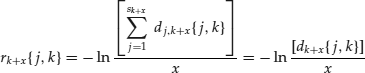
(28.1) ![]()
and, as a consequence of the absence of second-order arbitrage (the state constraints are all solved with equality), the following relationship may also be derived:
(28.2) ![]()
where Dt represents the m × 1 vector of dual prices with djt the dual variable associated with state j at time t. The vector of dual prices, Dt, is known commonly as the state price vector. Equations 28.1 and 28.2 represent a statement of the Fundamental Theorem of Asset Pricing (FTAP), a formal proof of which is contained in Prisman (1986).
The dual variables have the standard interpretation used in linear programming. If an investor is required to earn at least one unit of value in state j, the objective function increases by an amount djt. Accordingly, if a new security were to be defined with a value of one unit in state j at time t and zero in every other state, it must have a price equal to djt. Such an instrument is known as an Arrow-Debreu security.
When the number of independent securities, n, is equal to the number of states, s, at time t, the market is said to be complete. An important feature of a complete market is that the state values of any new security, including each of the s Arrow-Debreu securities, can be perfectly replicated by some portfolio of the original n securities, which, in order to preclude arbitrage, must be equal to the price of the replicating portfolio.
Only in the case of complete markets can unique prices be determined for all Arrow-Debreu securities. In markets that are incomplete, however, perfect replication is not guaranteed, and, in that case, only bounds can be placed on the prices of Arrow-Debreu securities.
PRICING RELATIONSHIPS
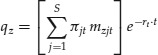
Assuming that the no-arbitrage condition holds in a complete market with no frictions, then the FTAP states that any arbitrary new security, z, must have the same price as a portfolio of Arrow-Debreu securities with holdings equal to the new security's value in each state as given by:
where mzjt is the value of the new security in state j at time t. Note that Equation 28.3 is equivalent to the replication approach described in the previous section, with the only difference being that, in this case, the replicating portfolio is comprised of the s Arrow-Debreu securities rather than the n original securities.
As a specific example, the risk-free security, f, with a guaranteed value of one unit at time t, by definition has a value of one in each future state, and must therefore have a price, qf, equal to:
where mfjt = 1 represents the risk-free security's constant value across all j states at time t and where the new terms dt and rt can be defined, respectively, as the discount factor associated with time t and the continuously compounded risk-free rate over a period of length t.
Inspection of Equation 28.3 reveals that by using the FTAP, any security can be priced without knowledge of either its expected time t value, E{mzjt}, or the individual state probabilities, pjt. This is a very important result. The implication is that the pricing of securities in a complete market requires neither the explicit modeling of an investor's attitudes toward risk, nor a description of the distribution of values across states. If it were necessary to model investor attitudes toward risk, it would require incorporating this statistical information, but in the complete market case the information is entirely embedded in the prices of the Arrow-Debreu securities. As a consequence, only the assumption underlying the no-arbitrage condition, the preference of more to less, is required for valuation purposes.
The fact that knowledge of state probabilities is unnecessary for valuation purposes motivates the risk-neutral valuation approach, so called because the valuations are independent of any assumptions made about investor attitudes toward risk. If investors were truly risk-neutral, the true expectation of any value distribution across states at time t could be discounted at the risk-free rate. However, since investors are not typically risk neutral, the true expected values cannot generally be discounted at the risk-free rate.
Nonetheless, we can get around this point. A simple algebraic manipulation of the FTAP defines, for each state j at time t, a new variable, πjt (defined such that ∑j=1s πjt = 1), that has the characteristics of a probability. From Equations 28.1 and 28.4, the magnitude of each πjt is calculated so that the pricing model can be viewed as discounting the risk-neutral expected value across states at time t, Mt πt, by the continuously compounded risk-free rate to return the correct price, or:
![]()
where:
![]()
and where πt represents the s × 1 vector of risk-neutral probabilities associated with states that occur at time t. As the result stems from a simple algebraic manipulation, and given that the true probabilities are not required for pricing, then the risk-neutral approach is appropriate regardless of an investor's true attitude toward risk. From Equations 28.3 and 28.4, the new security, z, can be alternatively valued under the risk-neutral technique as:
where πjt is the risk-neutral probability associated with state j at time t. In other words, we can say that the security's value is equal to the risk-neutral expected payment of the new security, discounted at the risk-free rate over time t.
PERFECT CAPITAL MARKETS
While the FTAP as developed in the previous sections relied explicitly on a single behavioral assumption, it also relied implicitly on three key assumptions underlying the dynamics of the market. These assumptions are described next and, along with the “preference of more to less” behavioral assumption, are typically referred to collectively as the perfect capital markets (PCM) condition. The combination of these assumptions ensures that the market operates efficiently from both an informational and an allocation perspective.
Frictionless Markets
Under this assumption, it is assumed that securities are perfectly divisible, meaning that they can be bought and sold in any fraction or multiple, and that there are no constraining regulations on trading, such as limits on short selling. In addition, it is also assumed that the market is free of transaction costs or taxes, although the no-taxation assumption can be relaxed if taxes are applied in a symmetrical manner, meaning that there is no differential taxation across investors.
Perfect Competition
Under this assumption, it is assumed that all investors are price takers, rather than price makers, and it ensures that no single investor can impact prices on the basis of the volume of the investor's trade. Equilibrium prices are assumed to result from the dynamics of the collective, as described by Adam Smith's “invisible hand” of market behavior. Another implication of this assumption is that there is always perfect liquidity in the market, implying that there are always as many buyers and sellers, and that prices adjust to clear the market without a liquidity premium.
Informational Efficiency
Under this assumption, it is assumed that all relevant information determining security prices is both costless and simultaneously available to all investors. In the context of the multistate framework described in the previous sections, this assumption implies that all possible future state values are known and agreed upon by all investors. Risk is modeled solely on the basis of the uncertainty of state occurrence, rather than on the uncertainty of security value given the realization of a given state.
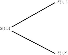
A TWO-STATE, SINGLE-PERIOD EXAMPLE
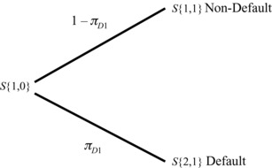
As an illustration of the model described earlier, consider the two-state model as shown in Exhibit 28.1 whereby the realized state j occurring at time-step k over time t is given by S{ j,k}. In this single time-step model, k = 1 for all future states over time t, while S{1,0} represents the current state known with certainty today.
Exhibit 28.1 Two-State, Single-Time-Step Model
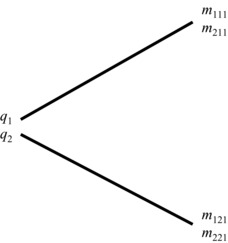
Consider two independent securities, priced today at q1 and q2, with state values of m111 and m211 occurring in S{1,1} and state values of m121 and m221 occurring in S{1,1}, respectively. Given that there are as many independent securities as there are states (n = s = 2), the implication is that the market is complete. It is also assumed that all assumptions underlying the PCM condition apply to this market. The state values of these securities are given in Exhibit 28.2.
Exhibit 28.2 Complete Market: Two Securities
Optimization Model
In this example, the behavior of arbitrageurs can be modeled by the following linear programming problem:
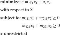
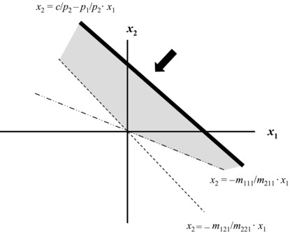
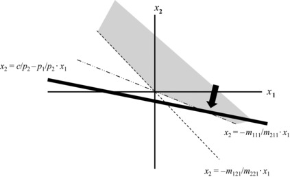
with the interpretation that the cost of a two-security portfolio is minimized, subject to the constraints that the portfolio's values must be nonnegative in each of the two future states in time-step 1. Graphically, the primal problem can be represented by Exhibit 28.3, where the dashed lines represent the boundaries of the two state constraints and where the shaded region represents the intersection of feasible solutions to the optimization problem in terms of holdings xi and xj. The heavy line represents the slope of the objective function, and the arrow represents the direction of cost minimization. The three cases of first-order arbitrage, second-order arbitrage, and the no-arbitrage condition are determined by the relative slopes of the three lines.
Exhibit 28.3 Feasible Region and Objective Function
In the case of first-order arbitrage, the slope of the objective function is either greater or less than the slopes of both of the lines representing the state constraints. In Exhibit 28.4, where m121/m221 > m111/m211 > q1/q2, assume that the (absolute) slope of the objective function is less than the (absolute) slopes of the constraints.
Exhibit 28.4 A Case of First-Order Arbitrage
In this case, the heavy line representing the objective function can be pushed infinitely beyond the origin (c becomes increasingly negative), as arbitrageurs will increasingly purchase security 1 and increasingly short-sell security 2 (x1 becomes increasingly positive and x2 becomes increasingly negative). The coordinates of the optimal portfolio will extend infinitely into the southeast quadrant, while the solution to the objective function is unbounded, as arbitrageurs reap unlimited first-order arbitrage unless prices readjust (i.e., unless the slope of the heavy line alters as q1 and q2 readjust).
In the case of second-order arbitrage, the slope of the line representing the objective function is equal to either of the slopes of the lines representing the state constraints. In Exhibit 28.5, where m121/m221 > m111/m211 = q1/q2, assume that the slope of the objective function coincides with state constraint 1.
Exhibit 28.5 A Case of Second-Order Arbitrage
In this case, the heavy line representing the objective function can be pushed only to the origin where the three lines intersect, and thus the solution is bounded (c = 0), implying that no first-order arbitrage profits are available. However, arbitrageurs can reap unlimited second-order arbitrage if state 2 were to occur, by increasingly purchasing security 1, and increasingly short-selling security 2 (x1 becomes increasingly positive and x2 becomes increasingly negative). The coordinates of the optimal portfolio will again extend infinitely into the southeast quadrant, this time along the coincident line of the objective function and state constraint 1 unless, once again, prices readjust.
In the case of the no-arbitrage condition, the slope of the line representing the objective function must be less than the slope of one state constraint and greater than the slope of the other. In Exhibit 28.6, where m121/m221 > p1/p2 > m111/m211, assume that the slope of the objective function is less than state constraint 2 and greater than state constraint 1.
Exhibit 28.6 A Case of Market Equilibrium
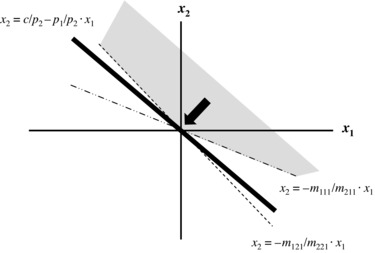
In this case, the heavy line representing the objective function can be pushed only to the origin where the three lines intersect and, thus, the solution is bounded (c = 0), implying that no first-order arbitrage profits are available. As the solution is solved with a single optimal portfolio (x1 = 0 and x2 = 0), there are also no second-order arbitrage profits available.
The key assumption underlying almost all pricing methodologies used in financial engineering is that observable prices available to investors are such that neither first- nor second-order arbitrage opportunities are available and, thus, case 3 must hold in market equilibrium. In other words, the behavior of arbitrageurs acting at the margin will serve to ensure that prices always readjust to achieve the no-arbitrage condition in equilibrium.
Fundamental Theorem of Asset Pricing
Given both the no-arbitrage condition and the assumption of a complete market in this example, the following relationships may be derived from Equation 28.1:
![]()
where d11 and d21 represent the unique prices of the Arrow-Debreu securities corresponding to states 1 and 2, respectively, at time-step 1 and are calculated as:
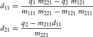
From Equation 28.3, the price of a new security, z, with values of mz11 and mz21 over states 1 and 2 at time-step 1, can be priced as a portfolio of Arrow-Debreu securities with holdings equal to the new security's values in each state. Therefore, in order to preclude arbitrage, the equilibrium price of a new security, qz, in market equilibrium must equal:
![]()
Applying the technique of risk-neutral valuation, the new security can also be priced by discounting its risk-neutral expected payment of (mz11 π11 + mz21 π21) by the risk-free rate over time t, or from Equation 28.5,
![]()
where:
![]()
INCORPORATING THE EVENT OF DEFAULT
The event of default can be incorporated into this general model as an occurrence within one or more states that triggers nonpayment of an agreed-upon value by the issuer of the security. An otherwise risk-free security, z, that exhibits default risk is one that has a value of one unit in each nondefault state and some recoverable amount, expressed in terms of a rate, 0 ≤ Φzjt ≤ 1, corresponding to each default state at time t.
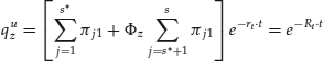
Assume that, of the s possible states at time-step 1, the first j = 1, … , s* represent nondefault of obligor (i.e., issuer) U while the remaining j = s* + 1, … , s represent obligor U default. For the moment, we also assume the market to be complete, implying the existence of n = s independent securities. Given that any security in a complete market can be replicated by a portfolio of Arrow-Debreu securities, then, from Equation 28.3, the price of a new risky security, quz, associated with issuer U must be:
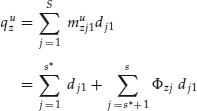
where muzj1 represents the credit-risky security's payment in state j at time-step 1, which in the case of nondefault muzj1 = 1, and in the case of default muzj1 = Φzj.
We now introduce a new variable, Rt that represents the continuously compounded risky discount rate associated with obligor U that can be used to price the credit-risky security over time t as:
where, in this context, the term risky refers to the default risk associated with obligor U.
From Equations 28.5 and 28.6, the price of the credit-risky security can be restated under the risk-neutral approach as:
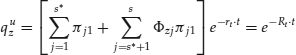
which provides a relationship between the risk-free discount rate and the risky discount rate. If we now make the simplifying assumption that the rate of recovery is constant across all states, then Equation 28.7 can be reexpressed as:
where Φz represents the recovery rate applicable to all default states for this security.
By now assuming a constant recovery rate, we can collapse the entire state space into just two super-states of default and nondefault where we can define the risk-neutral probability of default at time-step 1, πD1, as:
Accordingly, the risk-neutral probability of nondefault will be equal to, 1 – πD1, and this credit risk example can now be recast in the two-state framework as worked through in the previous section and as illustrated in Exhibit 28.7.
Exhibit 28.7 Two-State Model: Default and Nondefault
The advantage of the constant recovery assumption is that it now enables a complete market to be defined with only two independent securities required to span the default and non-default super-states. This can be achieved with just the risk-free and credit-risky securities as illustrated in Exhibit 28.8.
Exhibit 28.8 State Values of Risk-Free and Credit-Risky Securities
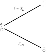
From Equations 28.8 and 28.9, the FTAP enables the price of the credit-risky security to be rewritten as:
Calculating a Credit Spread
We can define a credit spread as the difference between the risky rate and the risk-free rate, ρt = Rt – rt, for obligor U and, thus:
and, by further rearranging Equation 28.11, the credit spread corresponding to the period t = 1 can be expressed as:
or, when πD is sufficiently small, a Taylor Series expansion of Equation 28.12 allows the relationship to be more commonly defined as:
![]()
where the credit spread is shown to be a function of both the likelihood of default and the rate of recovery given default. Note that this relationship holds with respect to the risk-neutral probability of default as opposed to the true or statistical probability of default.
Inspection of Equation 28.10 reveals that the price of the riskless security must always be greater than that of the credit-risky security (qf > quz) or, alternatively, from Equation 28.12, that the credit-risky rate must always be higher than the risk-free rate (ρt > 0 or Rt > rt). This observation illustrates that a credit risk premium is always required for an investment in the credit-risky security, despite the fact that neither the statistical probability of default nor investor attitudes toward risk has been explicitly incorporated into the model.
The preceding result illustrates a subtlety associated with the conventional calculation of the required credit-risky rate and the credit spread. In classical finance, it is well accepted that a risk premium over and above the risk-free rate is required to entice a risk-averse investor to invest in a risky security. The overall required return is calculated on the basis of the statistical expected value at time t with respect to the current market price. This definition implies that the statistical probabilities of the occurrence of each state must be known in order to determine the expected value and, ultimately, the magnitude of the risk premium.
In contrast, the required credit-risky return, as defined in Equation 28.10, is calculated solely on the basis of the FTAP. Therefore, statistical state probabilities are not required in order to determine the magnitude of the credit risk premium. As a consequence, the credit risk premium, as conventionally calculated, does not arise out of an assumed trade-off between risk and return, but simply out of the no-arbitrage relationship derived from the “preference of more to less” assumption. In fact, the credit risk premium will always be positive, even in the case when investors are truly risk seekers.
A MULTIPERIOD FRAMEWORK
When the number of available states at a given time horizon, t, exceeds the number of independent securities, s, the market is said to be incomplete, as unique prices for Arrow-Debreu securities cannot be found and the FTAP cannot be used to uniquely price any arbitrary new security. Without either introducing sufficient independent securities to complete the market, or invoking an additional behavioral assumption, a refinement of the state process over time t must be made in order to determine unique Arrow-Debreu prices.
No-arbitrage pricing in markets that are not complete over time t can still be accomplished by imposing a multistep state process such that, at each state in an intermediate time step, the number of available states in the next time-step does not exceed the number of independent securities. Given such a state process, the market is considered to be “dynamically” complete over time t through a strategy of rebalancing holdings at each state in a given time-step, such that over any next time-step the market is always complete.
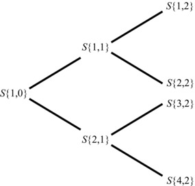
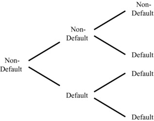
The lattice in Exhibit 28.9 illustrates a two-period, two-state process that represents a complete market in the dynamic sense. Although a total of four states is possible at time t, only two states are available over the first time-step and, contingent upon the realization of a given state in the first time-step, only two states become available over the second time-step. In this particular model, the overall time period, t, is divided into τ = 2 time-steps, whereby each future time-step is denoted by k = 1, … , τ and where k = 0 represents the known state today. The realized state j occurring in time-step k is represented by S{j,k}.
Exhibit 28.9 Two-State, Two-Time-Step Model
Extending the result of Equation 28.1, the FTAP in the multiperiod case can be expressed as follows:
where Q still represents an n × 1 vector of security prices, and where the sk × 1 vector Dk{1,0} represents the Arrow-Debreu prices observed in S{1,0} with future values corresponding to each state in a given time-step k > 0. The n × sk matrix Mk represents realized security values across each state of time step k with each matrix component, mijk, denoting the value of security, i, in S{j,k}.
Given a dynamically completed market, the S{j,k} observed price of an Arrow-Debreu security, with a value of one unit if state S{j,k + 1} occurs and zero otherwise, is always unique and equal to dj,k+ 1{j,k}. For the two-state, two-time-step framework described in Exhibit 28.9, the S{1,0} prices of both Arrow-Debreu securities associated with the first time-step are unique and equal to d1,1{1,0} and d2,1{1,0}, while the prices of the two contingent Arrow-Debreu securities observed in S{1,1} associated with the second time-step are also unique, and equal to d1,2{1,1} and d2,2{1,1}, respectively.
Likewise, the prices of the two contingent Arrow-Debreu securities observed in S{2,1} associated with the second time-step are unique and equal to d3,2{2,1} and d4,2{2,1}, respectively. Exhibit 28.10 illustrates the first time-step Arrow-Debreu securities and the prices of the contingent second time-step Arrow-Debreu securities associated with the framework described in Exhibit 28.9.
Exhibit 28.10 Contingent Prices of Arrow-Debreu Securities
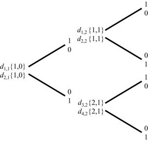
Exhibit 28.11 Prices of Arrow-Debreu Strategies
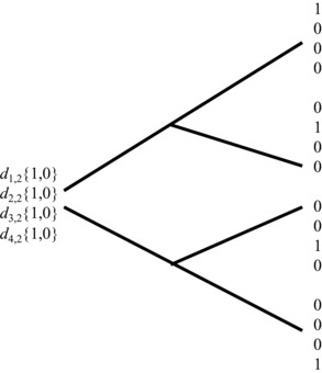
To preclude arbitrage in a dynamic context, the S{1,0} price of an investment that has a value of one unit in state j of the second time step and zero otherwise, dj,2{1,0} must be equal to the cost of the self-financing strategy of purchasing an Arrow-Debreu security at S{1,0} and rolling it over into the appropriate contingent Arrow-Debreu security that becomes available in S{j,1}.
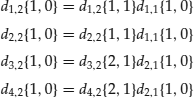
The price of the Arrow-Debreu strategy, d1,2{1,0} that produces a value of 1 in S{1,2} and zero otherwise, is achieved by purchasing d1,2{1,1} units of the Arrow-Debreu security associated with S{1,1} today and, contingent upon S{1,1} occurring, rolling the proceeds into one unit of the contingent Arrow-Debreu security associated with S{1,2}. The strategy is self-financing, as the d1,2{1,1} value of the investment reaped in S{1,1} is exactly equal to the price of the contingent Arrow-Debreu security associated with S{1,2}, and thus it must be the case that d1,2{1,0} = d1,2{1,1} d1,1{1,0}. Note, if instead S{2,1} were to occur in time-step 1, the investment would expire worthless. Exhibit 28.11 illustrates the prices of each Arrow-Debreu two-step strategy associated with the available securities illustrated in Exhibit 28.10, where:
The implication is that, in a complete and arbitrage-free market, any arbitrary new security must have the same price as a portfolio of the Arrow-Debreu strategies with holdings equal to the new security's payment in each S{j,k}. From Equation 28.13, the price of a new security, z, with state values of mzj1 and mzj2 over time-steps 1 and 2, can be priced as a portfolio of Arrow-Debreu strategies with holdings equal to the new security's values associated with each state over all time-steps. Therefore, in order to preclude arbitrage, the equilibrium price of a new security, qz, in market equilibrium must be equal to:
![]()
where, for k = 1, dj,1{1,0} represent the prices of the Arrow-Debreu securities analogous to a single period model and where, for k = 2, dj,2{1,0} represent the prices of the Arrow-Debreu strategies as defined earlier. In other words, any new security can be dynamically replicated through a series of single-step Arrow-Debreu securities.
By a simple algebraic manipulation of Equation 28.13, the risk-neutral valuation approach can be formulated for the multiperiod context in the following manner:
where:
![]()
represents an sk × 1 vector of the risk-neutral probabilities associated with each S{j,k} as observed in S{1,0}. The risk-neutral expected value of Mkπk{1,0} can, thus, be viewed as being discounted from each time-step k back to S{1,0} by the continuously compounded risk-free rate, rk{1,0}, associated with time-step k.
As a specific example, the risk-free security with a value of one unit across all states in a given time-step, k, must, therefore, have a price qf equal to a portfolio containing one of each of the sk Arrow-Debreu securities associated with time-step k or simply:
where, as before, mfjk = 1 represents the constant value of the risk-free security across all j states in time-step k, and where the terms dk{1,0} and rk{1,0} are defined, respectively, as the discount factor associated with time-step k and the continuously compounded risk-free rate over time-step k, both observed in S{1,0}.
Term Structure of Interest Rates
Note, in a multistep framework, that an arbitrary fixed income security, z, which makes constant payments across all states in each time-step k for multiple time-steps, must have the same price as a portfolio of risk-free securities with holdings equal to the fixed income security's payment in each time-step, or as per equation 28.15:
![]()
where mzk represents the constant payment of the fixed-income security across all states in time-step k.
If the security universe under consideration were to consist entirely of these fixed-income securities, then the multistep, multistate model collapses to a multistep, single-state model, which becomes exactly analogous to the multistate, single-time-step model described in the first section of the chapter. In this context, rather than solving for the prices of individual Arrow-Debreu securities for a single time-step, the no-arbitrage condition in complete markets (meaning here that the number of independent securities n equals the number of time-steps τ) enables us to solve unique discount factors for each time-step k. As the entire state space is now collapsed into a single super-state for each time-step, discount factors are solved for directly, rather than first solving for the prices of the Arrow-Debreu securities. This is the well-known bootstrapping exercise.
In a dynamically completed market (or in the static complete market of fixed-income securities just described), a term structure of “spot” risk-free interest rates can be defined, which, in the continuously compounded case, is expressed as:
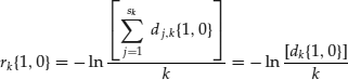
for a given term k.
Furthermore, in a dynamically completed market (this time a complete market of fixed-income securities alone will not suffice), it is also possible to define a series of contingent risk-free securities that are observed in some future S{ j,k > 0}. These securities can be priced for a given term x as observed in each future S{ j,k > 0} and will implicitly define a state process for the term structure of interest rates over τ time-steps such that the term structure can be expressed as:
for a given term x.
INCORPORATING DEFAULT
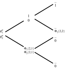
The event of default can be incorporated into the multi–time-step model as an occurrence within one or more S{ j,k > 0}, which triggers nonpayment of a commitment by the issuer of the security. Exhibit 28.12 illustrates the event of default for a given issuer as incorporated into the two-state, two-time-step framework described in Exhibit 28.10. Note that in this framework, default may occur immediately in step 1 or, alternatively, given that nondefault has occurred in time-step 1, it may then occur in time-step 2.
Exhibit 28.12 Default in Time-Steps 1 and 2
A given credit-risky security, z, issued by U, makes a fixed payment in each nondefault state and payment of some recoverable amount, Φz{j,k}, expressed in terms of a proportion of the fixed payment, in each default state. Exhibit 28.13 illustrates the prices, qu1 and qu2, and future payments of two credit-risky securities, one maturing in time-step 1 and the other maturing in time-step 2.
Exhibit 28.13 Payments of Credit-Risky Securities
A dash in a time-step 2 state indicates that the security has matured in a previous time-step. Note that, in addition to the possibility of defaulting at maturity, the two-time-step credit-risky security may now also default in the intermediate time-step. In this model, default is assumed to be an absorbing state as no resurrection of the two-time-step security is possible in the second time-step if default has occurred in the first time-step.
Given that any security can be replicated by a portfolio of Arrow-Debreu securities, then, from Equation 28.13, the price of the credit-risky security maturing at time-step 1, qu1, associated with issuer U must be:
![]()
where R1{1,0} represents the continuously compounded risky rate observed today over time-step 1.
While the pricing of the one-time-step credit-risky security is simply an application of the single-time-step model as described in the previous section, the pricing of the two-time-step credit-risky security introduces the complication of potential default prior to maturity. Again from Equation 28.13, the price of the zero coupon risky security maturing at time-step 2, qu2, associated with the same issuer U can be represented as:
![]()
where R2{1,0} represents the continuously compounded risky rate observed today over time-step 2.
Risk-Neutral Valuation
From Equation 28.14, the price of the zero coupon risky security maturing at time-step 1 can be restated under the risk-neutral approach as:
where Φ1{2,1} is the recovery rate given default associated with S{2,1}. The term πD1{1,0} = (1 – πD1{1,0}) represents the one-time-step risk-neutral probability of nondefault associated with S{1,1}, which can be expressed alternatively as the risk-neutral probability of survival until time-step 1.
Likewise, from Equation 28.14, the price of the credit-risky security maturing at time-step 2 can be restated under the risk-neutral approach as:
where πD2 is the risk-neutral probability of survival until time-step 2 and where πD∩D2 is the risk-neutral probability of time-step 1 nondefault followed by time-step 2 default. The recovery rate, Φ2{2,2}, is associated with time-step 2 recovery of default, given that no default occurs in time-step 1.
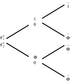
For analytical tractability, two typical, but perhaps unrealistic, assumptions are often made with respect to the multi-time-step case. The first is that recovery is pushed to the time-step of the anticipated payment (regardless of when default actually occurs), and the second is that the recovery rate is constant for each security issued by U and for all S{j,k}. Exhibit 28.14 illustrates the prices and values of the two credit-risky zero coupon securities resulting from these revised assumptions, where Φ represents the constant recovery rate associated with all default states at each time-step. In this context, Equation 28.17 can be simplified to produce a general relationship that resembles the specific one-time-step case of Equation 28.16:
Exhibit 28.14 Impact of Recovery Assumptions
Note that it is not generally the case that the risk-neutral probability of survival over x* time-steps, πDx*{1,0}, is equal to the risk-neutral probability of survival over x time-steps (where x* > x) multiplied by the conditional risk-neutral probability of survival over the next x* – x time-steps (πDx{1,0} · πDx*{D,x}). This observation relates to the fact that risk-neutral probabilities are simply an algebraic artifact and do not, in fact, represent true statistical probabilities. The condition that ensures equality of this relationship is independence of the interest rate process from the default process, which can also be satisfied by the stronger condition of nonstochastic interest rates.
Calculating the Credit Spread
The credit spread term structure, for each term k = x, can be defined as the difference between the credit-risky and risk-free term structures for issuer U or:
![]()
Given the modeling assumptions described earlier, then from Equation 28.18 the price of an x time-step credit-risky security issued by U must be:
![]()
implying that the spot credit spread for a term of x can be expressed as:
![]()
or when the risk-neutral probability of default over the next x time-steps is sufficiently small, by a Taylor Series expansion:
![]()
The credit spread in this context can now be simplified to an analytically elegant relationship that is a function of both the risk-neutral likelihood of survival over the next x time-steps, and the constant rate of recovery given default. See Das and Tufano (1996) and Duffie and Singleton (1999) for detailed formulations of no-arbitrage—based models for the pricing of credit risky securities
In the context of this chapter, this exercise illustrates a typical example of the modeling trade-offs often made to achieve mathematical nicety at the expense of economic reality. In practice, these tradeoffs often prove to be acceptable under normal markets conditions, but typically are the source of model breakdown under extreme events.
CONCLUSION
No-arbitrage pricing models are the most powerful valuation techniques used in financial engineering. As illustrated in this chapter, the only behavioral assumption required is that investors prefer more to less. Observable prices are assumed to be free of arbitrage as the actions of arbitrageurs, by seeking risk-free profits, push prices to an equilibrium state whereby all arbitrage opportunities are eliminated.
The unfortunate aspect of this, however, is that most of the market conditions necessary for its use are usually not present in the real world. Markets are rarely complete in the strict sense, and the required perfect capital markets (PCM) assumptions do not typically hold in practice. In addition, many other simplifying yet unrealistic assumptions (such as the constant recovery assumption used in the examples of this chapter) are often deployed for analytical tractability. Economic reality is often sacrificed to achieve mathematical elegance for modeling purposes.
Nonetheless, in competitive markets with appropriate liquidity and enough breadth to span a wide range of possible future states, no-arbitrage pricing models usually prove to be quite robust. By appropriately collapsing the entire state space into super-states (as illustrated in the bootstrapping and single-period credit spread examples), and by imposing exogenously defined state processes into the model (as illustrated in the multiperiod credit spread example), complete markets can be defined in a localized sense. Critical in all of this, though, is the appropriate specification of the securities’ joint value distributions across future states, capturing both the dispersion for each security and the co-dependence across securities.
The key challenge in the practical use of no-arbitrage pricing models is to understand when the underlying assumptions are appropriate and when they are not. In normal markets, where liquidity is plentiful and where the projected joint distributions across securities can be calibrated with confidence to the relevant past, the models usually behave quite well. In market dislocations, however, when liquidity can dry up and when correlations can converge to one, the underlying modeling assumptions must be reassessed or the models can fail dramatically.
In many cases, financial innovation in the markets has progressed faster than the mathematical tools required to adequately value new products, which is only magnified in times of market turmoil. While financial engineering has evolved significantly over the years by borrowing its mathematical techniques liberally from the physical sciences, the financial system is exposed to significant model risk if we ignore the fact that finance is fundamentally a behavioral science and not a physical science.
REFERENCES
Das, S., and P. Tufano. 1996. “Pricing Credit Sensitive Debt when Interest Rates, Credit Ratings, and Credit Spreads Are Stochastic.” Journal of Financial Engineering 5:2, 161–198.
Duffie, D., and K. Singleton. 1999. “Modeling Term Structures of Defaultable Bonds.” Review of Financial Studies 12:4, 687–720.
Prisman, E. Z. 1986. “Valuation of Risky Assets in Arbitrage Free Economies with Frictions.” Journal of Finance 41:3, 545–556.
Ross, S. 1976. “Risk, return, and arbitrage.” In Risk and Return in Finance, I. Friend and J. Bicksler, eds., 189–218. Cambridge, MA: Ballinger.
ABOUT THE AUTHOR
Andrew Aziz is executive vice president of Risk Solutions at Algorithmics, leading the firm's Buy-Side and Risk Analytics business lines. Andy has held a number of senior positions at Algorithmics, including vice president of products, vice president of professional services, and executive director of financial engineering. In addition, he currently teaches in the Financial Engineering Program at the Schulich School of Business in Toronto, Canada. Andy holds a number of degrees, including a PhD in finance from York University, an MBA in finance from Queens University, and a BSc (Honors) in chemistry from McMaster University.