
Chapter 8
The Commodity Market
Commodity Market Snapshot
History: Commodity markets pre-date recorded history, and their evolution was critical to the development of modern civilization. Early barter trades evolved into loosely organized markets, which then evolved into more organized markets. Today we have highly efficient cash and derivatives markets for most major commodities. The latter include both exchange-traded components and over-the-counter components. These markets continue to evolve with new electronic platforms rapidly replacing traditional open outcry.
Size: The growth in trading volume for both exchange-traded and OTC commodity derivatives has been impressive. The size of the exchange-traded markets, principally futures, is most often measured in terms of contract volume and contract open interest. The size of the OTC derivatives markets is most often measured in notional principals outstanding and gross market values. Notional principal in the OTC commodity derivatives markets grew from under $1 trillion in 1998 to almost $18 trillion 10 years later.
Products: The markets trade an array of products ranging from physical commodities for immediate delivery, to highly standardized exchange-traded products, such as futures and options on futures, that allow individuals and institutions to enter and exit positions quickly and efficiently. Customized derivative products are also available in the form of swaps and options. These products can be tailored to satisfy a host of end user needs.
First Usage: The first recorded futures trade was in rice contracts, developed in Japan during the seventeenth century. The over-the-counter commodity market developed during the 1980s when the first oil swap was introduced in 1986, with Chase Manhattan Bank as the intermediary in the transaction.
Selection of Famous Events:
Early seventeenth century: The first tulip bulbs were brought to Holland in 1559. A market that was dominated by the wealthy Dutch soon developed. However, by the 1630s, the middle-class of Dutch society began seeking out this coveted flower, resulting in escalating tulip bulb prices. The market ranged from those who purchased the flower for simple enjoyment to those who accumulated bulbs for the purpose of resale and generating profits. Prices reached their peak in 1636, and people began to liquidate their tulip holdings. Eventually, panic resulted and the tulip bubble burst, with prices declining by at least 90 percent within six weeks.
1993: Metallgesellschaft AG (MG), a German industrial conglomerate, revealed losses of $1.5 billion from its New York–based subsidiary, MG Refining and Marketing Inc. (MGRM). MGRM went long in energy futures and entered into OTC energy swap agreements to receive floating and pay fixed energy prices. However, a decline in energy prices, coupled with MG lacking sufficient funds to maintain their hedging positions, resulted in significant losses. Today, it is now a part of GEA Group AG, one of the largest system providers for food and energy processes.
2006: Amaranth Advisors, a Greenwich, Connecticut, hedge fund, made futures bets on natural gas prices to rise and leveraged those bets by borrowing money. Although the firm profited from the same speculative positions in the previous year, natural gas prices fell in 2006, causing Amaranth to lose about $6 billion.
Best Providers (as of 2009)
North America and Europe: Morgan Stanley.
Asia: Standard Chartered.
Applications: Some of the ways that investors may use commodity derivatives include hedging, short-term speculation, arbitrage, long-term investing, portfolio diversification, and building structured products.
Users: Commercial interests, including both producers and consumers of commodities, are active market participants. Increasingly, investors looking for alternative asset classes are being drawn to commodities as well.
HISTORICAL PERSPECTIVE
Commodities are at the heart of our very existence. We live in homes made of wood and brick. We wear clothes made of cotton and other fibers. We eat a breakfast of eggs, bacon, orange juice, coffee, and milk. We drive to work in a car made of a variety of metals and plastics and powered by gasoline or electricity. The commodities that we consume in our daily lives are ubiquitous; so much so that we simply take them for granted without giving them much thought.
Commodity markets have an extremely long history; indeed, they pre-date any written records. They were the first markets, existing even before there was money—at least, as we understand the concept of money today. Without trade in commodities, civilizations would not have developed and life as we know it today would not be possible. The earliest transactions in commodities took place tens, perhaps hundreds, of thousands of years ago and undoubtedly took the form of barter transactions between individuals of the same tribal band or between tribal bands that occasionally interacted. I might have caught a lot of fish; more than I can consume before the fish go bad. You might have killed some game and have more animal skins than you can wear. These situations, and hundreds like them, lend themselves to barter. Perhaps we can agree that 10 fish are worth 1 deer skin. So a trade is made.
The development of markets, initially through barter, but later using money, replaced the more brutal approach of taking what you want from others by force. As such, the development of commodity markets played a key role in the evolution of civilization. In time, people began to specialize in the commodities they produced, simply because people had different sorts of skills and preferences for the types of work they did. A good hunter is not necessarily a good fisherman. A good fisherman is not necessarily a good farmer. Thus people began to concentrate on producing those things wherein they had a comparative advantage and then traded their production for the production of others. The introduction of money, itself just a standardized commodity, greatly improved the efficiency of these early commercial transactions. Indeed, the introduction of money, in itself, was a truly astounding financial innovation.
Over time, markets became more organized. This might have taken the form of different tribal bands meeting annually at specific locations to trade with one another. In time, a merchant class began to develop, and they found that they could maximize their transactional volume and minimize their cost of transporting their goods, and thereby maximize their profit, by positioning themselves along natural trade routes. This pattern was repeated throughout history and explains why most of the world's major commodity markets are located where they are. Chicago, for one, was well positioned to become a center for trade in grains and related commodities because of its position on Lake Michigan and its proximity to the lush agricultural region known as the grain belt.
With the progression of time, merchants began to organize themselves into guilds. The guilds established rules of conduct that all members of the guild were expected to obey. These guilds, in turn, established more organized markets than had previously existed. They would set the times of market operation, develop standardized weights and measures, and designate trading and delivery locations. Because money (cash) was exchanged for commodities with immediate delivery expected, these markets became known as cash markets, though they are also known today as spot markets, actuals markets, and physicals markets.
As commercial interests grew in size and became more sophisticated, new needs emerged. For example, a miller might need 10,000 bushels of wheat to mill into flour every month because he has contracted to deliver that quantity of flour to a baker. But the cash market for wheat is only bountiful in supply at the time of harvest, and the miller does not have the resources to purchase a whole year's supply of wheat at one time, nor the storage capacity to warehouse that quantity of wheat. In response to these sorts of situations, grain merchants with access to storage would agree to sell wheat today for delivery at specific later dates; that is, dates “more forward” than were considered immediate. These contracts became known as forward contracts, and the early markets in them were made by some of the same merchants who marketed grains for immediate delivery.
Forward contracts were the precursors of futures contracts, but they were not supplanted by futures contracts. Instead, forward contracts and futures contracts co-exist as each has its advantages and its disadvantages. Most people believe that the Chicago Board of Trade (CBOT) was the first futures market, but it was not. The CBOT was established by grain merchants in 1848 and began trading futures in the 1860s. In fact, a futures market in rice had earlier existed in Osaka, Japan.1 It was known as the Dojima rice market, and it traded standardized futures-like contracts in the eighteenth century. Despite the fact that the Dojima rice market employed many of the same processes as were later employed by the CBOT, there is no evidence that the founders of the CBOT had any knowledge of this earlier rice market and its practices. Thus, futures trading, as an innovation, has occurred independently more than once. This speaks to the fact that a good idea is a good idea no matter who comes up with it. Today, futures markets exist throughout the world and employ similar structures and trading rules.
As commodity markets grew larger, they began to attract the attention of governments. When occasional shortages occurred, often due to the vagaries of weather, sharp increases in prices would result. Similarly, when the stars were aligned and Mother Nature cooperated, a bumper crop would bring so much supply to the market that prices would plunge. The former angered consumers, and the latter angered producers. Both sides would insist that speculators were manipulating the prices. Typically, they would refuse to accept that these price swings are natural market responses to imbalances in supply and demand and that they are the invisible hand that guides production and consumption. Such complaints, however ill-founded they might have been, eventually led to government oversight of these organized markets, which eventually became known as “exchanges” in some countries and “bourses” in others.
In the early days of futures trading, trading was confined to agricultural commodities—mostly grains and oilseeds, such as wheat, corn oats, and soybeans. In time, futures trading was extended to agricultural commodities other than grains and oil seeds. These included goods like coffee, cocoa, sugar, and cotton, and livestock products such as live cattle, pork bellies, and lean hogs. Still later, futures trading in non-agricultural commodities, such as industrial metals (e.g., nickel, aluminum, copper, lead, and tin) and precious metals (e.g., gold, silver, palladium, and platinum) were introduced. In more recent years, futures trading in a host of energy products, ranging from crude oil to natural gas to ethanol, was introduced. In time, it was realized that there was no real need to have a provision for physical delivery on a futures contract if acceptable and transparent cash settlement rules could be developed and enforced. This led to the introduction of non-deliverable (or cash settled) futures on both non-traditional commodities, such as freight rates and electricity, but also to futures on things that are clearly not commodities at all, such as stock indexes and interest rates.
In the 1980s, a number of important new developments occurred in the commodities markets, with two events standing out in particular. One was the introduction of exchange-traded options on futures, and the other was the introduction of commodity swaps and options. The former, like futures, are highly standardized contracts that trade on designated futures exchanges. The latter are over-the-counter (OTC) products that can be tailor-made (i.e., customized) to serve the specific commercial needs of end users. Some of the differences between exchange-traded and OTC commodity derivatives are important and will be discussed shortly.
Historically, few individual investors thought of commodities as “investment assets” except in the context of purchasing shares in commodity-producing companies. Physical commodities are, in most cases, simply too bulky to store and often have very limited life spans before they spoil. Futures, of course, represented an alternative way to take investment positions in commodities, but only a small segment of the investing community ever did so. Few had any real understanding of futures and futures market mechanics, and many of those who did feared the leverage built into these contracts. They were also often put off by the fact that most commodity futures have a relatively short life. In very recent years, however, portfolio managers and investment advisors have come to see commodities as an investable asset class—quite distinct from equities, fixed income, foreign exchange, and credit. In response to this growing acceptance of the concept of commodities as investments, and some clever financial engineering, a number of structured investment products have been introduced that any investor can use to gain exposure to commodities. Important among these are commodity-linked notes and commodity-focused exchange-traded funds. For wealthier investors, there are also “hedge fund”–like vehicles that specialize in commodities. These are known as commodity pools, commodity funds, and managed futures funds. Importantly, not all managed futures funds trade futures on commodities. Some trade futures on stock indexes, interest rates, and other non-commodity underlyings. In the United States, persons who run commodity pools must register with the Commodity Futures Trading Commission as commodity pool operators (CPOs) and persons who advise others on trading in commodities and who run individually managed commodity accounts on behalf of others must register as commodity trading advisors (CTAs). Both commodity pools and individually managed futures accounts are generally open only to investors who meet stringent criteria.
Collectively, these various engineered products have helped satisfy investors’ growing interest in commodities as investments in recent years. This new interest is driven, in part, by the view that commodities can be a good inflation hedge; in part by the fact that the inclusion of commodities in the investment asset class mix can improve diversification; and, in part, by the view that rapid economic growth in developing countries will continue to drive growth in demand that will, in turn, drive commodity prices higher.
EXCHANGE-TRADED VERSUS OTC COMMODITY PRODUCTS
It is common practice to divide commodity markets into “cash markets” and “derivatives markets.” The cash markets represent the markets where commodities can and are physically delivered following a transaction. The delivery may be immediate (immediacy is defined in the context of the specific market), or it can be for a period more forward than what is understood to be immediate. Contracts are negotiated directly between the buyer and the seller with all contract specifications spelled out in each contract drafted. These specifications include such things as the specific grade of commodity, the quantity of the commodity, the delivery date, the delivery location and mechanism, and the price, among other things.
The derivatives markets, which include both exchange-traded products and over-the-counter products, may or may not provide for physical delivery, and, in most cases where physical delivery is permitted, the contracts can be terminated without physical delivery, by either engaging in an offsetting transaction or negotiating a cancellation. The former include commodity futures and options on futures; the latter include swaps, cash-settled forwards, and OTC commodity options.
FUTURES CONTRACTS
Futures contracts only trade on designated futures exchanges. The exchange specifies all of the contract terms—everything except the price. Thus, the only thing that needs to be determined through the trading process is the price. The futures will be available in two or more delivery months. For example, there might be a June contract, a September contract, and a December contract. A person who wishes to buy a contract would contact his commodity broker and give appropriate instructions. He can place a variety of different types of orders but would most commonly use either a “market order” or a “limit order.” For example, a customer might say to his broker, “Buy 10 June gold at market.” Each of these contracts covers 100 ounces of gold, but prices are quoted in dollars per ounce. So his request translates to “buy for my account 10 June delivery gold futures contracts each covering 100 ounces of gold,” and he is willing to pay whatever current market conditions dictate. This is a market order because he is willing to pay the current market price. In this case, the current market price would be the best ask price (also known as an offer price) currently available. Had he specified the maximum price he is willing to pay, it would have been a limit order and the broker must get the limit price or a better price. If the broker cannot get the limit price or a better price, the trade does not occur. The same process works when selling a futures contract. For example, a customer might say, “Sell 5 June gold at $1275.40.” This is a limit order to sell five gold contracts, and the broker must get the customer a price of $1275.40 (or better) per ounce covered by the contracts. Importantly, one does not need to own a futures contract to sell one. The act of selling a futures contract creates a short position for the seller.
Both buyers and sellers of futures have to post margin with their brokers. Margin is typically 5 to 10 percent of the notional value of the contract, but the margin rules can vary depending on what other positions the customer simultaneously holds. If the price moves against the customer, he or she will be asked to post additional margin. If the price moves in the customer's favor (i.e., up for longs and down for shorts), the customer can withdraw money from his or her margin account.
Futures trading is symmetric in that there are exactly the same number of contracts held long as held short (i.e., one person's long position is another person's short position). Thus, the profits earned by one person come at the expense of losses to the other person. In the language of economics, this makes futures trading a “zero sum game.” Importantly, it is only a zero sum game in a “monetary profit/loss” sense. In terms of economic “utility,” futures trading can be win-win for both parties.
A customer can get out of a futures position with ease. If he is long a contract, he simply sells a contract of the same delivery month, and he is out. If he is short a contract, he simply buys a contract of the same delivery month, and he is out. This ease of entry and exit is made possible because of the standardization of contract terms and the intermediation of the clearinghouse.
Affiliated with every futures exchange, but still distinct from the exchange itself, is a clearinghouse. The clearinghouse becomes the counterparty to the customer on every trade he does, no matter with whom he traded. That is, the customer who buys a contract is “long to the clearinghouse” and the “clearinghouse is short to the customer.” By the same token, a customer who sells a contract is “short to the clearinghouse,” and the “clearinghouse is long to the customer.” Thus, if a customer initially bought 10 June gold futures, he is long 10 contracts to the clearinghouse. If he later sells 10 June gold futures, he is then short 10 contracts to the clearinghouse. Because his counterparty in both cases is the clearinghouse, his positions cancel. He is left with the gain or loss that results from the difference between the price at which he bought and the price at which he sold. Those prices were determined on the exchange when the transactions were made.
The employment of clearinghouses and the posting of margin are key elements of futures market mechanics. The clearinghouse is protected from market risk because it is always long and short the same number of each contract. It is protected from credit risk by the margins posted by the position holders. Because of the relatively small amount of margin posted by customers, futures afford traders enormous leverage. For example, if the margin requirement is 5 percent of the notional value of the contract, the customer has leverage of 20 to 1. This is great when markets move in your favor but can prove devastating when prices move against you—hence the phrase, “leverage is a double-edged sword.”
Participants in the futures markets include members of the exchange and the trading public. Here we refer to the latter as customers. Included among the members of the exchange are market makers. These exchange members offer to buy futures contracts at one price and to sell the same contracts at a slightly higher price. They are the principal, but not the only, source of market liquidity. They look to profit from the small difference between their bid (buying) price and slightly higher ask (selling) price. As noted earlier, ask prices are also known as offer prices. Other exchange members try to earn their livings by exploiting short-term trends in the price or by spotting and exploiting inefficiencies in contract pricing. Customers, and those are our real interest here, may be individuals, commercial entities such as corporations, or investment pools of various sorts. Some are short-term speculators, others are longer-term investors (the dividing line between speculators and investors is completely arbitrary), some are hedgers, and others are arbitrageurs. Speculators and investors attempt to profit by correctly predicting the direction of the market price and then positioning themselves to profit from the coming price change. Hedgers, in contrast, take positions in futures to offset the risks associated with other positions they presently hold or anticipate that they will later acquire. For example, a feedlot operator who has contracted to buy 500 calves, with delivery to be made a few months after the next birthing cycle, knows that he will need a certain amount of corn as feed to raise the calves before slaughter. His fear is that the cost of corn may go up before he takes delivery of the calves—thereby increasing his production costs. To hedge himself, he buys futures now with delivery dates after the point where he would take delivery of the calves. When he takes delivery of the calves, he goes into the cash corn market, purchases the physical corn that will be used to feed the calves, and simultaneously terminates his long futures positions by offsetting transactions. He may wind up paying more or less than he originally anticipated for the cash corn, but this unanticipated loss or gain is offset by the profit or loss on the futures contracts he used to hedge his anticipated future corn needs. Notice that he did not need to take delivery on the futures for the hedge to work, provided that the spot price of corn and the futures price of corn are sufficiently highly correlated.
Arbitrageurs seek to earn profits by exploiting perceived price discrepancies in markets. As a simple example, suppose that in August, an arbitrageur observes that the current spot price of corn is $3.80 per bushel. He also observes that the November corn futures price is $3.95 per bushel. He knows that it will cost him $0.02 a month per bushel to store corn for a total of $0.06 in storage costs. He will also have to absorb $0.03 per bushel to transport the corn and $0.03 per bushel to finance his holdings of the physical corn. Thus, he can buy the physical corn for $3.80, absorb total costs of $0.12 for storage, transport, and financing for a total all-in cost of $3.92. Simultaneously, he sells futures at $3.95, thereby locking in a riskless profit of $0.03 a bushel. There are many other types of arbitrage scenarios; some, like this one, are conceptually simple, while others are far more complex. But do not be fooled; futures markets are highly efficient, and true arbitrage opportunities are very rare.
Historically, futures trading was conducted on the floors of large futures exchanges in what are called “trading pits.” Each pit traded futures in one commodity but in multiple delivery months. Trading was conducted through a combination of voice and complex hand signals. Because pits take up a lot of room, the number of commodities that could be traded was limited by the size of the trading floor. Over the last few decades, futures trading has moved into the electronic age. The transition from physically meeting on a trading floor to meeting and trading in cyberspace was traumatic for many of the exchange members, and many resisted the transformation. But, the old does, sometimes reluctantly, make way for the new, and today most futures trading is conducted electronically. Indeed, some futures exchanges have completely retired their trading floors, and others are destined to eventually do so. This transition itself was an exercise in financial engineering, and it brought both greater speed to execution and a reduction in trading errors (i.e., miscommunications between buyers and sellers). It also made it possible to introduce futures on many additional commodities and non-commodities, as floor space became less of an issue.
Options on futures work the same way that equity options work, which are discussed in other chapters of this book, so we will not elaborate on them here, except to say that options on futures come in both call and put varieties and the “deliverable” is the specified underlying futures contract. Delivery of the futures contract would only take place if the option contract is exercised. The buyer of the contract pays a “premium” up front to the option writer (i.e., the seller) for the right that the option conveys. Specific option pricing models have been developed for options on futures. These models are similar to, but still not the same as, the models used for valuing equity options. The drivers of an option's value include the current price of the underlying, the volatility of the price of the underlying, the strike price of the option, the life of the option (i.e., the amount of time before the option expires), and the level of interest rates.
RISK MANAGEMENT WITH COMMODITY FUTURES/OPTIONS
There is a long literature on the use of commodity futures and, to a lesser extent, options on futures as risk management tools. Risk management is a science, a subset, so to speak, of the field of financial engineering, and it takes considerable study to do it well. Nothing illustrates this point better than a commodities hedging disaster that, in 1993, befell Metallgesellschaft AG (MG), a German industrial conglomerate. In that year, the company revealed that it had suffered losses of $1.5 billion on hedged positions in energy futures. Essentially, the company had sold over-the-counter energy derivatives and then hedged those positions by going long energy futures. Unfortunately, the correlation of the energy futures prices to those employed in the OTC market was less than expected, and, when oil prices plunged, MG was faced with massive margin calls. MG is an important case study in many university risk management and financial engineering programs precisely because it made a series of mistakes in both structuring its hedges and in managing those hedges.
COMMODITY SWAPS
Commodity swaps are an excellent example of how an innovation in one market can be recycled and become an innovation in another market. The first true swap (as distinct from earlier transactions that had similar cash flows but different contractual and legal structures) was a currency swap. This was done in 1979. The first interest rate swap was done in 1981. These early swap markets were “brokered” markets in which a bank, acting in the capacity of a broker, would match two counterparties having similar but opposite requirements. In exchange for its services, the bank would collect a commission from both end user counterparties. This commission was often referred to as “structuring fee.” At first, these markets grew slowly, but when the broker banks realized that they could greatly facilitate swap transactions by transforming themselves from brokers to dealers, the swaps market took off. By 1986, the dealer market structure was well established, and, in that year, financial engineers (though that term had not yet been coined) at Chase Manhattan Bank (now part of JPMorgan Chase) realized that there was no apparent economic reason why a similar swap structure could not be applied to commodities. Typically, today, one counterparty to a commodity swap is a dealer and the other is an end user, but both parties can be dealers, and both parties can be end users. End users are parties other than dealers who have some commercial purpose for doing a swap.
In a plain vanilla commodity swap, one counterparty agrees to pay a fixed price per unit on some notional quantity of commodity. For example, consider an oil company in Texas that pumps 300,000 barrels of a specific grade of crude oil per month at the rate of 10,000 barrels per day. Each day, the company is credited with that day's spot price for its grade of oil for all the oil it pumped into the pipeline that day. Suppose now that the current spot price for the company's grade of oil is $70.50 per barrel. Its production costs are $55 per barrel. Management's worst fear, of course, is that the oil price might decline below the company's production cost, forcing the company to shut down its wells. Unfortunately, if the company shuts down its wells, it may not be able to start them up again, potentially forcing the company to pump at a loss until it is bankrupt. The company's monthly profit diagram or risk profile, with respect to the price of oil, is depicted in Exhibit 8.1.
Exhibit 8.1 Profit Diagram or Risk Profile
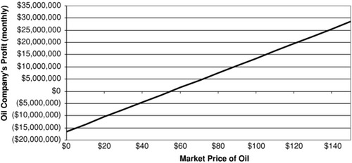
Exhibit 8.2 Oil Swap Hedge Application
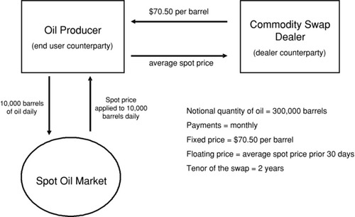
To remove this risk, the company's risk manager decides to enter into a two-year oil swap, in which the company will receive a fixed price of $70.50 per barrel once a month on 300,000 notional barrels of oil, from a swap dealer, at which time it will pay to the swap dealer the “average spot price over the prior 30 days” on the same notional quantity of oil.2 The oil swap together with the cash market transactions are depicted in Exhibit 8.2.
It should be plainly obvious that this commodity swap is structured a little differently from most interest rate and currency swaps that you may have seen. Those types of swaps typically make one observation per payment period on the floating leg side. In this swap, the floating side takes the form of the “average spot price” from daily observations on the market price for oil. It is this average that is paid monthly on the 300,000 barrels. We could, of course, have simply made one single observation on the spot price of oil on a specific day of the month—the first business day of the month, the 15th of the month, or the last business day of the month. But, because the oil producer sells its output daily, none of these would give it a perfect hedge. That is, the single monthly observation could be more than it received or less than it received, on average, for its oil over the course of the month. By averaging the observed spot price over the course of the month, the correlation between what the company received in the cash market for oil and what it pays out on the swap will be much higher. The higher the correlation, the more effective the hedge. With this structure, the oil company can be confident of netting $15.50 per barrel profit on each of its 300,000 barrels of monthly production. That is, it has locked in a monthly profit of $4,650,000 for the next two years. The principal cost to the company is that it has also traded away the “upside,” which is the potential to make even greater profits if the price of oil were to rise from its current $70.50 level.
These swaps can also be used to speculate and to invest, and also can be used as inputs in the construction of a variety of structured products and strategies. We will see several applications of this later. Importantly, the same banks that make markets in commodity swaps also, typically, make markets in commodity forward contracts.
COMMODITY OPTIONS
Many of the same dealers who make markets in commodity swaps also make markets in commodity options. Like options on futures, these can be calls or puts. They can be structured to be physically deliverable or cash settled. We will assume cash settlement for purposes of this discussion. Consider a call on oil. An end user buying the call would agree up front on the option's strike price, the notional quantity of oil, the settlement date, and the method and timing of observing the spot price for purposes of calculating the final settlement. The option will “pay off” at expiration based on the following formula:
![]()
Had the option been a put, the payoff formula would have been:
![]()
Where max is the maximum function and denotes the larger of the possible value of the term in brackets. S denotes the spot price observed in the manner agreed upon, X denotes the strike price of the option, and NQ denotes the notional quantity of oil (i.e., the number of barrels the contract is written on).
The call will “pay out” at the end if and only if it is in-the-money at its expiration. This would require that S > X. Otherwise, the call will pay out nothing. Similarly, the put will “pay out” at the end if and only if it is in-the-money at its expiration. This would require that S < X. The purchaser of either option will pay the dealer a premium up front and may lose some or all of this premium. But in no case will the option purchaser lose more on the option than the premium paid.
Using the same oil company described earlier in the swap hedging example, we will this time hedge the oil producer's risk exposure using an option. For the moment, we will assume that the oil company only wishes to hedge one month's production.
As noted earlier, the spot price of oil happens to be $70.50. The oil company, again, does not wish to take the risk of a decline in the price of oil, but doesn't want to hedge its risk with a commodity swap because, by so doing, it surrenders the opportunity to profit even more if the price of oil were to rise.
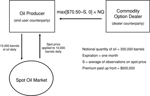
So, the company's risk manager approaches the commodity option dealer, and the dealer prices up a put option hedge on oil. They agree that the notional quantity of oil will be 300,000 barrels. They further agree that the option will pay off in precisely one month based on an average of the daily observations of the spot oil price— just as could have been done with the swap. They further agree that the strike price of the option will be $70.50. For this option, the dealer wants an up front premium of $2.00 per barrel covered, which means the option will cost the oil company $600,000. The structure, for just the one month life of the option, is depicted in Exhibit 8.3.
Exhibit 8.3 Oil Option Hedge—Put
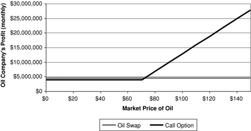
Now suppose that the average spot price of oil over the course of the month turns out to be $60.50 a barrel. The oil producer earns $1,650,000 from its transactions in the cash market. This is calculated by taking the price $60.50 that it received for its oil in the cash market, deducting the company's production costs of $55.00 per barrel, and multiplying by 300,000 barrels. But, at the same time, the company's option pays off because the put is in-the-money. The payoff is $3,000,000. However, because the company paid $600,000 up front for the put option, its profit on the option is only $2,400,000. Combining the profit of $1,650,000 earned in the cash market with the $2,400,000 profit earned on the option, the company's hedged profit for the month is $4,050,000. This is the company's worst case scenario and its overall profit would have been exactly the same at any oil price at or below $70.50. The reader is asked to verify this on his or her own. The beauty of the option hedge becomes obvious if the price of oil rises rather than falls. Suppose, for example, that the spot price of oil averages $78.50 over the course of the month. Then the company's overall profit for the month would have been $6,450,000; and if the price of oil had averaged $82.50 over the course of the month, the company's overall profit would have been $7,650,000. Again, the reader is invited to verify these numbers on his or her own (don't forget to deduct the premium paid for the option).
The oil company's profit diagram using the option hedge is contrasted to the oil company's profit diagram using the swap hedge (but just for the first month) in Exhibit 8.4. These should be compared to the profit diagram/risk profile with no hedge depicted in Exhibit 8.1. More experienced readers will notice that the profit diagram associated with the option hedge resembles the payoff profile of a call option, even though we employed a put as the hedging instrument. This is a manifestation of what is known in the option literature as “put/call parity.”
Exhibit 8.4 Comparative Hedged Profit Diagrams: Swap versus Option
Before closing this section, consider how the oil company might have hedged its production of oil out to a full two years as it did with the swap. The company could have purchased a series of 24 separate put options. The first would have a one-month expiry and would pay off based on the average spot price observed in the first month; the second would have a two-month expiry and would pay off based on the average spot price in the second month, and so on. Each of these options would command its own up-front premium. All other things being equal, the longer the time to expiry, the more expensive the option will be. But rather than purchase 24 separate options, each with a different expiry, and each for a different premium, dealers will offer a pre-packaged multiperiod option called a “commodity floor” that accomplishes the same thing at the same up-front cost. A floor is simply a portfolio of individual puts. The individual puts, in which the floor can be decomposed, are known in the trade as “floorlets.” While not shown here, the same is true for calls. A package of commodity calls structured to pay off at regular intervals over a period of time is called a “commodity cap,” and the individual option components of the cap are called “caplets.”
Exhibit 8.5 OTC Commodity Derivatives Notional Amounts Outstanding
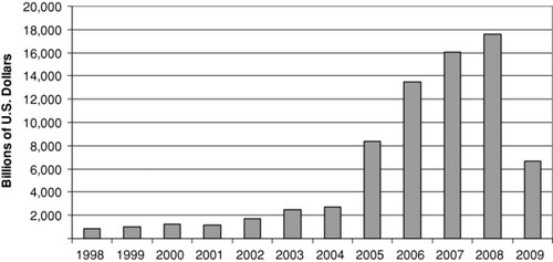
Exhibit 8.6 Over-the-Counter Commodity Derivative Market by Instrument (1998–2009)
Source: All data provided by Bank of International Settlements (BIS).
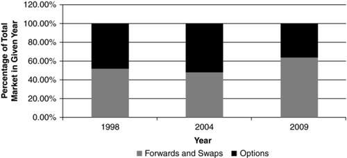
It is interesting to consider how the OTC commodity derivatives markets have grown. As indicated in Exhibit 8.5, total notional principal outstanding grew from less than $1 trillion in 1998 to almost $18 trillion in 2008, before declining sharply in 2009. It is also interesting to compare the makeup of the notional principal in terms of the percentage that is represented by options and the percentage that is represented by swaps. The swap figure also includes forwards (which can be viewed as a subset of swaps). This is depicted for select years in Exhibit 8.6. All data included in Exhibits 8.5 and 8.6 is drawn from the Bank for International Settlements (BIS).
FINANCIAL ENGINEERING IN COMMODITIES MARKETS
All the products we have looked at, as well as the commercial strategies that employed them, represented, at one time or another, financial innovations by financial engineers. The people who thought up these products did not use the term “financial engineer” to describe themselves, as that term came later. They just saw themselves as thinking creatively and outside of the box. We will now consider some recent financial engineering used to create commodity-based investment products.
Investment Products
As noted earlier, one of the first commodity-based investment products, other than futures contracts themselves and the holding of physical commodities, were managed futures funds, also known as commodity pools. These did not begin to become popular until after 1974. As a general rule, they are only opened to sophisticated investors, defined loosely as those with significant net worth or significant income. Generally, in the United States, investors must be either “accredited,” as that term is defined by the SEC, or a “qualified eligible person,” as that term is defined by the CFTC, in order to qualify for participation in a commodity pool.
The commodity pool operator may take a technical approach to the trading of commodities, a fundamental approach, attempt to engage in arbitrage, or some combination of these. Early commodity pools tended to take a technical approach, and most still do. By technical approach, we mean they use technical analysis that depends on past patterns of price behavior to anticipate future price behavior.3 This approach is heavily focused on spotting trends, and then positioning the pool on the right side of a trend. Typically, the commodity pool will hold positions in many different commodity futures simultaneously and may be long on some commodities while short on others. This diversification gives the pool some benefit in the form of risk reduction. Effectively managing a commodity pool requires that attention be paid to the management of cash. This is necessitated by the considerable leverage these funds employ and the need to meet daily margin requirements.
One of the great attractions to introducing commodities into an investment asset allocation plan is that commodities, as a group, tend to have relatively low degrees of correlation with more traditional asset classes, such as stocks and bonds. It is well understood that diversification, as a risk reduction tool, only works well when the assets that are collectively held have relatively low correlations with one another. Indeed, for many, this is the single biggest attraction for considering commodities as an investment.
Commodity-Linked Notes
We will focus here on exchange-traded commodity-linked notes. These are a subset of both exchange-traded notes and structured notes. (Structured notes will be discussed more broadly in other chapters of this book.) Importantly, not all exchange-traded notes or structured notes have a commodity component, but some do. When they do, they are said to be commodity-linked.
Exchange-traded commodity-linked notes trade, oddly enough, in equity markets, in exactly the same way as stocks trade. While the trading mechanics are identical, the tax and accounting rules can be quite different, and the investor needs to be aware of that. These notes are, most often, issued by highly rated banks. They typically take the form of a non-interest bearing bond that pays off at maturity based on the performance of a given commodity or a given commodity index. Most often, they are principal protected, so that the investor is guaranteed to recover the par value of the note at maturity, but they don't have to be. The principal guarantee is achieved by, essentially, coupling a zero coupon bond with a commodity option. These products typically have a life of a few years, three to seven being most common, but there are similar products with much shorter maturities as well.
The commodity-linked note can be structured to reward an investor who believes that a particular commodity will rise in value over the life of the note or fall in value over the life of the note. That is, they come in varieties that allow investors to express both bullish and bearish views on commodity prices. We'll consider one of each.
Suppose that a particular AA+ rated bank would like to raise some capital by tapping into investors’ interest in commodities as an investment. Suppose further, that the bank has determined that there are many investors who are bullish on gold, and who would like to gain some exposure to gold, but who do not want downside risk. Similarly, the bank has determined that there are also some investors who are bearish on gold and who would also like to gain exposure to gold (from the short side), but who also do not want the downside risk. So the bank tasks its financial engineering department (which can go under many different labels) to engineer products to satisfy these two groups. Suppose the bank wishes to raise $200 million from “bullish on gold” investors and $100 million from “bearish on gold” investors. Suppose further, that the bank would like three-year funding and is prepared to pay 3.228 percent per annum, compounded annually. That is equivalent to 10 percent over three years when the compounding is taken into consideration.
To satisfy the bullish-on-gold investors, the financial engineers realize that all they need to do is have the bank purchase an appropriately structured three-year gold option. Suppose that the current price of gold is $1250 an ounce. The bank buys a three-year cash-settled gold call on 160,000 ounces of gold. This would be purchased from an OTC commodities derivatives dealer. The number of ounces of gold was determined by dividing the total to be raised, $200,000,000, by the current price per ounce, $1250. This option will pay off at the end of the three-year period based on the spot price of gold at that time. In order to be certain that the bank does not pay more than 10 percent of the funds to be raised (i.e., $20,000,000) for the option, they need to do a few calculations. First, on a plain vanilla $200 million zero coupon bond, the interest of $20,000,000 would have been paid three-years out.4 But the option premium must be paid up front. Therefore, the $20,000,000 must be discounted to its present value. Discounting at a flat 10 percent, this is $18,181,818. Next, divide this by 160,000, which is the number of ounces of gold covered by the option. The result is $113.64. The trick is now to find the strike price for a three-year gold call that will result in a per ounce option premium of $113.64. All other things being equal, the higher the strike price, the lower the premium paid for a call option. However, other factors, such as gold-price volatility, will also play a role. Let's suppose that if the strike price is set at $1362.50, the option can be obtained for $113.64.
The bank then issues a $200,000,000 non-interest bearing note that guarantees to pay the sum of $200,000,000 + (max[G3 – $1362.50, 0] × 160,000), where G3 denotes the spot price of gold at the maturity of the note, to the collective holders of the note at maturity. The option that the bank purchased is simply a hedge against its promise to redeem the note at maturity for a sum that includes appreciation, if any, in the gold's price beyond $1362.50. The structure is depicted in Exhibit 8.7.
Exhibit 8.7 Structure Underlying a Bullish-on-Gold Commodity-Linked Note

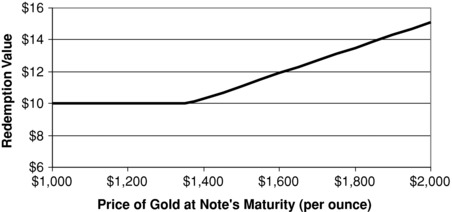
While the total note issuance is for $200,000,000, the note is actually sold in small denominations, which we will refer to here as units. Suppose that these are $10 each. Each unit entitles the holder to a pro-rata share of the final payoff at maturity. The note would likely be described, in the prospectus or offering circular, a bit differently than we described it here for ease of investor comprehension. For example, instead of working in dollars per ounce of gold, we could do the following: Since the current price of gold is $1250 and the option strike price is $1362.50, the price of gold would have to rise by 9 percent from its price at the time of the note's issuance before the gold-linkage contributes to the redemption payout. Thus, the investor would be told that, for each unit owned, he or she will receive, at the note's maturity, a sum given by: $10 +(max[A% – 9%, 0] × $10). The investor will receive no coupon interest, but will benefit from a significant rise in the price of gold without any risk to his or her principal. A payoff diagram at maturity is typically included in the prospectus so that the investor can better understand, at a more intuitive level, his final payoff. This is depicted is Exhibit 8.8.
Exhibit 8.8 Redemption Value at Bullish-on-Gold Note Maturity per $10 Invested
In this example, the issuer achieved its objective of raising capital at the targeted rate of 3.228 percent per annum with no risk to the bank from a change in the price of gold, despite the fact that it had embedded a gold call in its note. This was possible only because the note issuer is fully hedged with respect to gold. Both parties are pleased with the outcome.
Importantly, as the recent financial crisis that racked the global banking community so clearly demonstrates, well-rated bank issuers can get themselves into serious difficulty in a remarkably short period of time. Lehman Brothers and Bear Stearns were both big issuers of these sorts of notes. Lehman Brothers’ note investors are creditors of the bank, and it is doubtful that they will recover the full par value of their investment as that company winds its way through bankruptcy proceedings. This, however, is a manifestation of credit risk and has nothing whatsoever to do with the structure of the commodity-linked note.
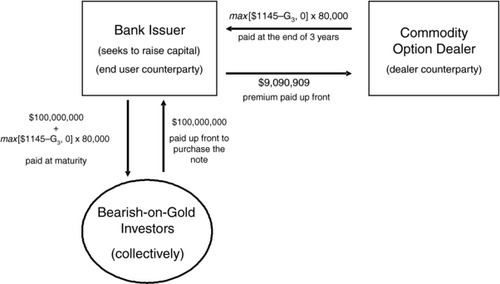
Just as our bank issuer tapped into a desire by some bullish-on-gold investors to express their view on gold without taking downside risk, so too can we structure a note to appeal to bearish-on-gold investors. This would require that the bank issuer hedge with a put option, rather than a call option, and then embed a gold put into the note it issues. Recall that the bank sought to raise $100,000,000 from this latter group. Assuming, for simplicity, that the appropriate strike price for the gold put is $1145 in order to hedge the dealer and achieve a funding cost of 3.228 percent per annum, the dealer would promise a per unit redemption (assuming an issuance price of $10 per unit) given by:
![]()
From the bank's perspective, the structure of the overall note (not on a per unit basis) is given in Exhibit 8.9. The notation used in Exhibit 8.9 should be interpreted in an identical fashion to that used in Exhibit 8.7.
Exhibit 8.9 Structure Underlying a Bearish-on-Gold Commodity-Linked Note
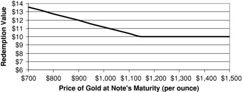
The payoff to the bearish-on-gold investors at redemption would be illustrated in the prospectus and would look something like that depicted in Exhibit 8.10.
Exhibit 8.10 Redemption Value at Bearish-on-Gold Note Maturity per $10 Invested
Importantly, the financial engineering we did here in order to help our issuing bank raise the capital it needs could be expanded to include oil-linked notes, or silver-linked notes, or even an index-of-commodities-linked note. Consider, for a moment, the latter. There are a number of important commodities indexes that could be used. Two of the most popularly quoted are the Dow Jones-UBS Commodity Indexes and the CRB Commodity Index (CRB denotes the Commodity Research Bureau). We build notes linked to an index by hedging in index-linked call or put options from a commodity options dealer.
We could also get more exotic, if we wished, by combining different options to create more unique commodity-linked payoffs at redemption. For example, we could structure bullish-on-gold-linked notes that employ a “gold collar” rather than a simple call. Or we could structure a note that paid off at redemption based on the “better performing” of several different commodities by using basket or rainbow options to hedge the issuer's exposure. More complex structured notes and the options used to hedge them are discussed elsewhere in this book, so we will say no more here on the subject.
From the bank's perspective, each investor's desire to express his or her view represents a “liquidity bucket.” The more of these liquidity buckets a bank can tap into, the easier it is to raise capital cost effectively. Investors are generally willing to accept a slightly lower implicit rate of interest in order to get a structure that fits their investment view, and the bank is rewarded by lower overall-funding costs.
COMMODITY ETFS
As a final thought on financially engineered vehicles that can be used by investors, small investors, in particular, (often referred to as retail investors or individual investors) may consider an exchange-traded fund (ETF) approach. Exchange-traded funds, which are discussed in considerable detail elsewhere in this book, were first introduced in 1993 to make available to the public a simple cost-effective and tax-efficient vehicle for investing in the broad market. The first ETFs were based on the S&P 500 index and are generally known as “spiders.” When an investor buys a share of spiders, he or she has, effectively purchased an interest in the entire S&P 500. Later innovations include an ETF on the Dow Jones Industrial Average, known as “DIAMONDS,” and an ETF on the Nasdaq 100, known as “Qs” (because of the ticker symbol). Later, sector-specific ETFs began to appear, which held only stocks representing a specific industrial sector. Since their debut in 1993, literally hundreds of ETFs have been introduced and today, trading in shares ETFs represents a very high percentage of total daily stock trading volume.
Over the past few years, financial engineers have extended the concept of an ETF to commodities. There are some commodity ETFs that are broad-based, similar to an index of commodities, and others that are single-commodity based. Without a doubt, the single largest of this latter segment are gold ETFs, which come in several different forms. Behind many ETFs is a “trust structure” that issues “units,” that investors can trade with both long and short positions. The units represent undivided claims in the pool of assets held by the trust—similar in that sense to a mutual fund. While there are several different legal structures that can underlie an ETF, all ETFs work in basically this way. In the case of gold ETFs, there are some that hold physical gold bullion, with the units representing indirect claims on this bullion, and others that hold stock in gold mining companies and, in that sense, are similar to sector-specific equity ETFs.
There is no doubt that ETFs are one of the most popular financially-engineered products. Commodity ETFs are particularly appealing to smaller investors who are unsuited to use futures markets and who have no interest in taking on the credit risk associated with commodity-linked notes, but who still want to express a commodity view.
REGULATION OF COMMODITY MARKETS
While regulation will vary from country to country, in most countries futures markets are regulated by the same governmental entity that regulates securities markets. For example, in the U.K., this is the Financial Services Authority (FSA). But in the United States, futures trading has its own regulator, the Commodity Futures Trading Commission (CFTC), which is separate and distinct from the principal regulator of securities markets, the Securities and Exchange Commission (SEC). Irrespective of this difference, futures markets, wherever they occur, are highly regulated. OTC commodity derivatives markets, on the other hand, are not as heavily regulated. Further, the degree of regulation of the OTC commodity derivatives markets varies considerably from country to country.
A FINANCIAL ENGINEERING EXERCISE: SYNTHESIZING BARTER
In an odd twist on history, financial engineers have demonstrated how commodity derivatives, particularly commodity swaps, can be used to create synthetic barter.5 The simplest structures, applicable when the two commodities trade in the same currency, can be achieved by combining two plain vanilla commodity swaps that have been properly “sized” so that the fixed-pay legs cancel. The payments on the floating legs are then used to offset the floating prices (i.e., spot prices) paid or received for the commodities in their respective cash markets. When the currencies in which the commodities trade are different, the solution becomes more complicated. In these cases, a fixed-for-fixed currency swap (i.e., a “cross-currency swap”) must be added to the mix. These transactions can be beneficial when a country is heavily dependent on the export of a particular commodity—such as oil in the Middle East.
The irony here is that we have come full circle. Commercial transactions began with barter. But barter was not efficient. Yet, through properly structured (i.e., engineered) commodity derivatives we can replicate or synthesize barter. And, as has been shown by those same financial engineers, though it is not shown here, the swap-synthesized barter solution ameliorates the problems associated with actual barter. The reader is encouraged to try to synthesize barter by appropriately labeling the arrows in Exhibit 8.11. Think of Country X as your client.
Exhibit 8.11 Exercise: Label All the Arrows to Create Synthetic Barter
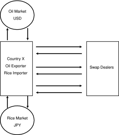
Scenario: Your client, County X, is an exporter of oil and an importer of rice. The oil is sold in the world's oil markets for U.S dollars. The rice is purchased in Japan for yen. Country X is exposed to three different market risks: the price of oil in dollars, the price of rice in yen, and the price of dollars in yen (i.e., exchange rate risk). Country X wants to lock in a fixed price for rice in terms of a fixed quantity of oil, such that the same amount of oil will be required to acquire the same amount of rice each month for the next five years. You have been asked to structure a synthetic barter arrangement that accomplishes this objective. In structuring your solution, don't worry about the actual prices of oil, rice, or the exchange rate. Just map out the set of transactions, on behalf of your client, that would be necessary to achieve an outcome equivalent to a given quantity of oil for a given quantity of rice. Importantly, the two parties would buy and sell their actual oil and rice in those commodities respective cash markets. They would not exchange oil directly for rice. After you have completed this exercise, you might want to read the reference noted in this section to check how you did.
NOTES
1. For a history of futures trading in Japan, see Hauser (1974).
2. We often use the term “notional quantity” to refer to the number of units that a commodity derivative is written on. Most people prefer to measure the size in terms of notional principal. The notional principal is simply the market price times the notional quantity. Notional quantity is used here for ease of exposition.
3. Technical analysts often employ more than just past price behavior in their effort to identify the future direction of an asset's price. They often employ volume, open interest, and other “transactional” data.
4. If an analogy were being made to zero coupon Treasury bonds, the bonds would be thought of as having a face value of $220 million and sold at issuance for the discounted price of $200 million. At maturity (i.e., redemption) the investors would collect the $220 million.
5. Marshall and Wynne (1996).
REFERENCES
APX, Inc. 2008. “Creating a Trusted Environmental Commodity.” www.apx.com/documents/APX-Trusted-Environmental-Commodities.pdf.
Benhamou, Eric, and Grigorios Mamalis. 2010. “Commodity markets (overview).” Book Articles: Forthcoming in the Encyclopedia of Financial Engineering and Risk Management. www.ericbenhamou.net/documents/Encyclo/commodity%20markets%20_overview_.pdf.
Celent. 2009. “ Commodity Markets: New Rules for a New Game.” www.celent.com/124_1103.htm.
Commodity Online India Limited. n.d. “What Is a Commodity Market?” Learning Center. www.commodityonline.com/learning_sub.php?id=5.
DeCovny, Sherree. 2010. “Commodities on the Rebound.” Market View: A Magazine for the Exchange Industry, June 22. www.nasdaqomx.com/whatwedo/markettechnology/marketview/marketview_2010_2/commodities_rebounding/.
Doyle, Emmet, Jonathan Hill, and Ian Jack. 2007. “Growth in Commodity Investment: Risks and Challenges for Commodity Market Participants.” FSA Markets Infrastructure Department. Financial Services Authority, March. www.fsa.gov.uk/pubs/other/commodity_invest.pdf.
Futures Technology. “History of the Commodity Markets.” 2010. History of Commodities, April 9. www.futurestech.net/history.htm.
Garner, Carley. 2010. A Trader's First Book on Commodities. Upper Saddle River, NJ: Pearson.
Hauser, W. B. 1974. Economic Institutional Change in Tokugawa Japan. London: Cambridge University Press.
Holmes, Frank. 2010. “The Case for Commodities in 2010 (and beyond).” Resource Investor, January 25. www.resourceinvestor.com/News/2010/1/Pages/The-case-for-commodities-in-2010.aspx.
Investopedia ULC, 1999. Investopedia. www.investopedia.com.
Marshall, John F. and Kevin J. Wynne. 1996. “Synthetic Barter: Simulating Countertrade Solutions with Swaps.” Global Finance Journal. 7: 1, 1–12.
Mlost, Karol. 2007. “Commodities futures pricing and approximation of convenience yield for Brent and WTI crude oils.” Master's Thesis. Wyzsza Szkola Biznesu–National-Louis University.
Oxford Futures, Inc. 2009. “A Brief History of Commodities.” Futures Fundamentals. www.oxfordfutures.com/futures-education/futures-fundamentals/brief-history.htm.
“Semiannual OTC Derivatives Statistics at End-December 2009.” BIS Statistics. Bank of International Settlements. www.bis.org/statistics/.
Thinking Finance. 2009. “Commodity Market Overview.” ThinkingFinance.net. www.thinkingfinance.net/commodities/56-commodity-market-overview.html.
U.S. Department of the Treasury. 2009. “Administration's Regulatory Reform Agenda Reaches New Milestone: Final Piece of Legislative Language Delivered to Capitol Hill.” Press Room: U.S. Department of the Treasury. www.treas.gov/press/releases/tg261.htm.
United Futures Trading Company, Inc. 1997. “The Basics of Commodity Futures Trading.” United Futures Trading. www.unitedfutures.com/commodities-trade.htm.
United Nations. 2010. “Recent developments in key commodity markets: trends and challenges.” United Nations Conference on Trade and Development, January 12. http://www.unctad.org/en/docs/cimem2d7_en.pdf.
Ward, Kurtis J. n.d. “The Futures Industry: From Commodities to the Over-the-Counter Derivatives Market.” KIS Futures. www.kisfutures.com/pdf/FUTURESINDUSTRYlawpaperKurtisWard.pdf.
ABOUT THE AUTHORS
Helen Lu is currently a second-year undergraduate student at Princeton University and plans to pursue a BA degree in Economics with a Certificate in Finance. Her academic interests include economic history, focusing especially on significant financial losses, and analyses of the recent global financial crisis. She has been working with the financial advisory firm, SBCC Group, on various financial engineering research projects that focus on risk management and on the history of financial engineering and financial institutions. She has also been involved in organizations intended to educate young women in smart and practical investment strategies in the financial markets.
Cara M. Marshall is a professor of finance at Queens College of the City University of New York. Cara holds a Ph in Financial Economics from Fordham University and an MBA with a focus on Quantitative Analysis from St. John's University. Her research interests focus on financial engineering, risk management, and derivatives, as well as behavioral and experimental methods in finance. Cara's Ph dissertation examined the pricing of volatility on U.S. options exchanges. Prior to academia, Cara worked in internet engineering, developing websites and a platform for online course delivery. She has also worked as a marketing manager for a conference and training company. Over the years, Cara has consulted to several investment banks as a trainer. In this role, she taught financial modeling to bank employees in New York, London, and Singapore. Cara has also performed analysis for hedge funds and for firms in other industries.