Chapter 14

Independent Valuation for Financially-Engineered Products

Cindy W. Ma and Andrew MacNamara

Houlihan Lokey

INTRODUCTION

Financial engineering has led to the creation of a wide variety of financial vehicles. Many of these are complex, making the analysis and risk management of these products more difficult than “plain-vanilla” investments. However, there are many situations that call for valuation, including portfolio management (whether to buy or sell an investment at a given value), financial reporting (including net asset value calculation), and dispute resolution. In these circumstances, it is often critical to develop a thoughtful, flexible valuation model backed up with well-researched input assumptions, and to present an analysis of multiple potential scenarios. Because of the complexity of these tasks and the amount of judgment required to analyze financially-engineered products, it is often advisable to seek an independent party (i.e., other than the portfolio managers or the members of the deal team) to help provide valuation advice. While some larger institutions have the resources to develop an internal group that provides independent views, third-party support can provide both small and large institutions with needed analytical support and independence.

Transparency has been a key issue for market participants throughout the financial crisis that started in 2007. Whether decrying the complexity of relationships between giant financial institutions or implementing rules meant to increase disclosure requirements, both investors and regulators have indicated that transparency is critical. For example, the recent Dodd-Frank Wall Street Reform and Consumer Protection Act requires central clearing of certain over-the-counter derivatives, along with data collection and publication in a section appropriately titled “Wall Street Transparency and Accountability.” Indeed, financially-engineered products are often esoteric, bespoke, or complex. Independent valuations can be one element of a strategy designed to improve the price transparency for these instruments.

In this chapter, we investigate the world of financial engineering, giving some examples of these kinds of products along with various analytical methods and considerations for valuation and risk management. Finally, we argue that the complexity of many financially engineered products, and the amount of judgment required in evaluating the choice and application of valuation models, suggest that third parties can provide independence and transparency to the valuation process, which is critical in many circumstances.

THE UNIVERSE OF FINANCIALLY ENGINEERED PRODUCTS

What are financially-engineered products? Let us first examine the field of financial engineering. According to the International Association of Financial Engineers (IAFE), “financial engineering is the application of mathematical methods to the solution of problems in finance.” This statement gives a sense of the breadth of topics the field covers. While the categorization of “financially engineered products” may be disputed, some of the papers that appear on the IAFE's website discuss such products as credit derivatives, collateralized debt obligations (CDOs), insurance, and commodity derivatives. In addition, other topics that have been addressed include systemic, market, and liquidity risk, as well as hedge fund return attribution.

Accounting standards have been trending toward greater use of market data in financial reporting for some time. While Accounting Standards Codification (ASC) Topic 820, “Fair Value Measurement,” has generated a significant amount of press coverage, it introduces relatively few new concepts.1 ASC Topic 820 does not prescribe when assets or liabilities should be measured at fair value, but it does define fair value. It also gives a framework as to how fair value should be measured and requires certain additional disclosures. Therefore, ASC Topic 820 is a key source document for financial reporting and valuation issues.

ASC Topic 820 defines fair value as “the price that would be received to sell an asset or paid to transfer a liability in an orderly transaction between market participants at the measurement date.” It clarifies that the price should not represent a distressed liquidation or other forced transaction, and contemplates a “usual and customary” exposure to the market to allow for marketing activities. “Market participants” are buyers and sellers who are independent of the reporting entity, have a reasonable knowledge of the asset or liability, and are both willing and able to transact for the asset or liability.

THE FAIR VALUE HIERARCHY

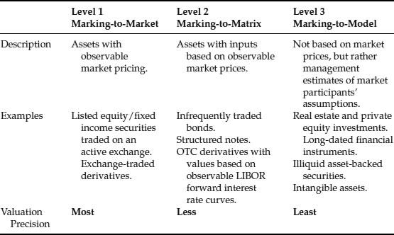
ASC Topic 820 requires the measurement of assets and liabilities using three hierarchical levels of input assumptions:

As shown in Exhibit 14.1, Level 1 deals with assets with observable market pricing while Level 3 is the most subjective. As such, the valuation precision generally decreases as the level increases.

Exhibit 14.1 Fair Value Hierarchy

Valuation of financially engineered products involves many different types of mathematical analytical techniques. For example, according to a model described by Hull and White,3 the valuation of a credit default swap (CDS) involves estimating expected probabilities of default based on bonds issued by the reference entity and then computing the present value of the expected payments and payoffs on the swap. On the other hand, valuing traditional CDOs can involve simulations based on copulas, which model the joint distributions of several variables (in this case, the probabilities of default of the underlying bonds). In addition, derivatives valuation procedures today often incorporate a credit value adjustment,4 which is intended to capture the risk that the counterparty to the transaction will not make good on its commitments. Many financially engineered products, especially highly complex, bespoke instruments, would fall under the Level 3 category for valuation purposes under ASC Topic 820.

Valuing financially engineered products can be challenging. First, financially engineered products are often esoteric or bespoke; they often are not well-covered by academic research, and as a result the models used to value them may not capture certain relevant features or may break down under certain market conditions. Second, much of the valuation technology developed to analyze these products involves models that contain simplifying assumptions designed to allow traders to obtain valuations quickly; however, these “black box” models can sometimes obscure important modeling assumptions that should be considered carefully in the context of a valuation. As a result, analyzing these products requires a careful evaluation of the facts and circumstances surrounding the product to see whether and how standard modeling practices can be applied and where they fall short.

MODELING ALTERNATIVES: CDOS

One example of the importance of scrutinizing accepted valuation models involves CDOs. These products were developed in the late 1980s. In general, a CDO raises capital in the form of debt and equity and invests it in a portfolio of financial securities. Conceptually, CDOs redistribute the risks and returns on a portfolio of collateral according to certain structural rules. Initially, CDOs focused on funding the purchase of portfolios of corporate debt, but as the product matured, other forms of collateral were used, including corporate loans, commercial real estate, and trust-preferred securities. Structured finance or asset-backed security CDOs (SF CDOs or ABS CDOs) invest in portfolios of securitized products, including mortgage-backed securities of different kinds, and sometimes liabilities, or “tranches,” issued by other CDOs.

Like other forms of securitizations, CDOs usually contain provisions designed to allocate credit risk (i.e., minimize the risk of principal loss to the most senior tranches). One of these provisions is structural subordination—in general, senior tranches receive principal before junior tranches, and junior tranches absorb losses before senior tranches. Exhibit 14.2 illustrates structural subordination and another credit risk protection used in other securitized products, overcollateralization,5 in a generic asset-backed structure.

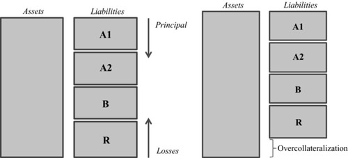
These charts illustrate structural subordination (left) and overcollateralization (right). The different CDO liabilities are labeled with different names that correspond to differing levels of seniority: for instance, the Class A1 notes are shown as senior to the Class A2 notes and so on. The “R” class denotes the residual, or equity of the deal, which is usually structured to receive any excess cash flow generated by the assets.

In addition, CDOs often include trigger tests, which can affect the distribution of cash flows among tranches and, in so doing, provide additional protection to senior tranches. For ABS CDOs, these are often in the form of overcollateralization (OC) tests and interest coverage (IC) tests. OC tests are defined at the tranche level and measure (in general) the ratio of the par amount of non-defaulted collateral to the par amount of outstanding debt for a given tranche.6 The higher the ratio, the more note holders are protected from credit loss.7 IC tests are also measured at the tranche level and compare the ratio of the scheduled interest due on the underlying collateral to the scheduled interest due on the given tranche and all tranches senior to that tranche. Again, the higher the ratio, the more protection the senior note holders have. These ratios are periodically tested against predefined trigger levels. If the ratio does not meet the trigger, interest proceeds from the collateral are diverted; instead of paying interest on junior tranches, the interest that would have been paid on those tranches is used to pay principal on the senior tranches. Since the interest is not paid in cash on the junior tranches, they are sometimes referred to as pay-in-kind tranches.8

In general, the more junior tranches of a CDO are more risky, since they bear losses before the more senior tranches and can also have interest paid in-kind instead of in cash. For the equity in a CDO, the risk may be more nuanced. CDO equity cash flows can be concentrated toward the end of the life of the deal; once the principal of the debt tranches is paid off from the amortization of collateral assets, the equity is entitled to the remaining collateral value, including any excess spread that has built up over the life of the deal (of course, CDO equity is also the first to bear losses on the collateral).

Traditional modeling techniques for CDOs focused on assessing the probabilities of default of individual collateral assets and the correlations of those defaults. For example, many market participants use a Gaussian copula model for estimating the probabilities of default of the CDO portfolio and, in turn, the CDO tranches themselves. Extensions of this concept include the use of “base” correlation mapping, which infers a correlation parameter from observable market data in a similar way that implied volatilities are calculated for traded options based on the Black-Scholes option pricing model. However, this technique has seen much negative publicity in the wake of the financial crisis starting in 2007. It is argued that some of the simplifying assumptions of the model itself, like the normal distribution assumption, do not reflect reality and lead to dramatic underpricing of risk because the model does not give sufficient weight to the incidence of highly-correlated, elevated default rates in times of market stress.

How can an analyst reconcile the elegance and market-wide use of these mathematical models with a fundamental understanding of the shortcomings of the model? One important first step is to return to basics: understand the key assumptions of the model, under what circumstances they can make the model results less useful, and how critical they are. Once this understanding is established, additional steps can be taken to evaluate or mitigate the model's shortcomings. For example, the distribution of defaults between similar assets could be measured, and the chances of a severe downturn that would cause highly-correlated, elevated defaults estimated. A more rigorous investigation would involve the construction of different models that do not rely on the same modeling assumptions; valuation results should be corroborated by these models.

Valuation Methodologies: Cash Flow Analysis

For example, one alternative to copula models that has been used by many analysts of CDOs (especially ABS CDOs) is a discounted cash flow (DCF) model. One of the key valuation steps in performing a DCF analysis of securitized products is developing reasonable assumptions about the expected future cash flow characteristics of the underlying assets. The cash flow characteristics of a pool of securitized assets are generally affected by factors such as prepayment rates, delinquency rates, default rates, and loss severity.

Prepayment rates refer to early repayments of a loan by a borrower.9 Prepayments are generally paid out to senior tranches before junior tranches, so an increased amount of prepayments will affect senior tranches and junior tranches differently. The more prepayments a given deal experiences, the shorter the life of the senior tranches will be; this can result in a higher value (if the bonds are already trading below par) or a lower value (if the bonds are already trading above par) based on straightforward bond mechanics. However, if a deal experiences an increased level of prepayments, junior tranches will not be able to benefit from an increased level of excess spread from those prepaid loans. Therefore, increased prepayments may in fact be detrimental to the value of junior tranches.10

Delinquency is the percentage of the loan pool that is late in paying scheduled payments by a certain amount of time and the loan is termed “delinquent” by a certain number of days (e.g., 30–59 days delinquent, 60–89 days delinquent, etc.).

Default rates are rates at which borrowers default, or fail to satisfy their obligations, on their loans.11 Since defaults generally result in some recovery of principal for the loan holder when the underlying collateral is sold, defaults usually result in an early repayment of principal on the underlying collateral. However, unlike other forms of prepayments, default liquidations often result in accompanying losses if the liquidation proceeds are insufficient to repay the loan. Therefore, liquidation proceeds are usually used to pay down senior tranches while losses are applied against the credit enhancements at the lower end of the capital structure (e.g., overcollateralization and junior tranches). For a senior tranche, then, an increased level of default can result in increased principal payments in the near term, which can be beneficial to senior debt holders. However, if built-up losses exhaust the credit enhancements on a senior tranche, the principal of the tranche can be affected by losses as well; once collateral losses reach this point, increased defaults will result in lower cash flows to the senior tranches; this, in turn, may result in lower values for those tranches. Since junior tranches generally absorb losses before senior tranches and often do not receive prepayments, increasing default levels usually result in lower values for these tranches. These relationships are highly dependent on the waterfall structure of the deal.

Loss severity measures the amount of loss on a defaulted loan's principal experienced upon the liquidation of the underlying property.12 The lower collateral values fall, the lower the amount of liquidation proceeds that are available to the trust; and consequently the higher the loss severity. Also, for loans that hold a second or higher lien on the underlying collateral, liquidation proceeds are applied to the first-lien loan before proceeds are available to pay the junior-lien loan. Therefore, loss severities are generally much higher on these junior-lien loans than on first-lien loans, often approaching 100 percent or more (e.g., costs incurred in the foreclosure process build up over time, and since they are often paid upon a liquidation of the underlying collateral before the junior-lien loans, the calculated loss severity on those junior loans can exceed 100 percent).

Significant resources have been dedicated to estimating the projected future cash flow performance of pools of securitized collateral. In the case of residential mortgage loans, analyses range from simple extrapolations of historical performance trends to state-based roll-rate models that project the probabilities of given borrowers entering different payment states (e.g., from current to paid off, or from current to 30 days delinquent) to detailed loan-level econometric models. Insights from the latter types of studies have revealed the connection between macroeconomic variables and loan performance (e.g., when interest rates decrease, voluntary prepayments tend to increase as borrowers refinance their loans early; also, when home prices decline, recovery rates on defaulted loans also decline, since the reduced proceeds from the sale of the collateral are used to satisfy the claim of the lender). Regardless of the specific projection methodology chosen, it is important to test the assumptions through comparative analysis: Are the near-term projections consistent with recent historical performance? Are the projections internally consistent (e.g., if the collateral includes a large population of delinquent loans, the default rates should be expected to increase)? Are there fundamental characteristics of the collateral being adequately captured (e.g., the projections should reflect rate resets on adjustable-rate loans)? Are macroeconomic trends or conditions being captured (e.g., loan modification programs)?

In addition to forming a reasonable set of loan pool projections, it is often helpful to incorporate multiple scenarios to capture different possible outcomes of loan performance.

Scenario Analysis

Many financially-engineered products incorporate the concept of financial leverage in their structures, either explicitly (as in the tranches of CDOs) or implicitly (derivatives positions can be used as vehicles for obtaining leveraged exposure to underlying investments). In the context of credit risk, leverage acts to increase the “tail risk” of the investment. An extreme example can be seen in a mezzanine tranche of a CDO: These subordinated tranches were often structured as very thin pieces of the capital structure. If losses erode all the credit support below a given tranche, any incremental loss may represent a large percentage write-down on the tranche, even though it may represent only a small loss relative to the size of the collateral pool as a whole. Because of this, loss outcomes can be viewed as almost “binary” for some tranches of these types of CDOs: Losses are either nonexistent, if collateral losses do not erode the credit support, or they are total, if collateral losses result in a write-off of the tranche itself.

For investments that incorporate this type of leverage, evaluating multiple scenarios is especially important. In this way, the analyst can gain an understanding of the sensitivity of the investment's potential cash flows under various plausible scenarios as well as under a worst case and a best case scenario. In some cases, the analyst will assign probabilities to each of the scenarios he or she has created, and weight the value indications from each according to its estimated probability of occurring. In addition, the range of outcomes is also important: If the performance of a leveraged investment is especially sensitive to small, plausible changes in input assumptions, an investor may require additional returns relative to a less-sensitive investment.

It may seem that we have taken a circuitous route from stochastic copula models, which incorporate various probabilities of assets defaulting, to cash flow analysis that is driven by a single set of projections, to scenario analyses, which incorporate multiple projections with different probabilities. However, it is important to remember that the reason to explore alternative models is to address potential deficiencies in existing valuation models. If a scenario-based cash-flow analysis is based on the same fundamental assumptions as the copula model, the analysis will not help address these potential deficiencies.

In addition, thinking about the valuation of a given asset in the context of a different analytical model sometimes highlights different characteristics of the asset that may not be captured well by a given model but that play an important role in valuation. This may help identify risks affecting the investment that may be measured and managed. Also, if a particular valuation model does not incorporate a given risk factor, the model cannot be used for managing the risk of the investment related to that particular factor. This is another benefit of using multiple models to analyze financially-engineered products.

INCORPORATING THE EFFECTS OF ILLIQUIDITY IN VALUATION

Another important factor to consider in valuing financially engineered products is illiquidity. Many of the more esoteric, bespoke, or complex financially engineered products would need to be evaluated using Level 3 inputs under ASC Topic 820. As discussed earlier, Level 3 input assumptions require valuation assumptions not based directly on market evidence. With financial investments whose value is dependent on a significant amount of judgment, the effects of liquidity are important to capture: the risks inherent in that judgment are amplified when the investor cannot easily sell the investment if necessary (i.e., if the investment is illiquid). Therefore, when analyzing a financially engineered product, it is important to capture the effects of the liquidity of the investment.

Liquid assets, such as equities traded on exchanges, are generally much easier to value than illiquid assets. Their worth can usually be determined based on observed transactions that occur between willing buyers and sellers. Illiquid assets are difficult to value because of the absence of transaction data. A fundamental analysis of the value of an illiquid asset is necessary. While liquidity risk is well understood and accepted, even from a common-sense standpoint, its full impact is not always recognized in valuations. For example, the term “liquidity risk” can be applied both to asset liquidity risk (i.e., the risk of not being able to sell an asset because of a lack of volume in the market) and funding liquidity risk (i.e., the risk of a company being forced to liquidate assets because of a lack of available funds). Funding liquidity risk can come into play with leveraged investments, which may draw a margin call when valuation levels fall. Faced with a margin call, an investor is forced to put up cash or sell the investment, sometimes at a considerable loss.

The Global Financial Crisis Exposed the Illiquidity Risk of Financially Engineered Products

The two forms of liquidity risk are intertwined. Declines in one form of liquidity can lead to declines in the other. This was seen vividly during the global financial crisis starting in 2007, when market participants were painfully on the “misery-go-round:” (i) asset values dropped quickly, causing an upheaval among banks, structured investment vehicles, and much of the securitization market; (ii) leveraged entities were forced to liquidate assets to meet margin calls; (iii) the resulting excess supply of assets drove down their values further; (iv) lower asset values forced further margin calls; and the misery cycle continued. Even companies that avoid leverage can face funding risk. When other counterparties cannot finance the purchase of assets through capital markets, demand for the assets can fall, leading to declines in asset values.

The value of illiquidity has been observed in many anecdotal situations throughout the recent financial crisis. Many investors that formerly purchased financially-engineered products (whether structured products, auction-rate securities, or complex, bespoke derivatives transactions) have “fled the market” and no longer invest in these products. The prices of some of these products have gone down despite low estimated credit risk, suggesting that investors value liquidity.

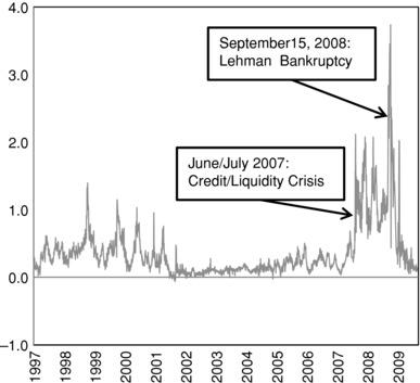
Exhibit 14.3 contains a chart of the historical yield spread between the 3-month AA-rated financial commercial paper and 3-month constant-maturity Treasury. This measure has been used as an indication of market-wide liquidity. During the summer of 2007, short-term debt (such as the commercial paper issued by financial institutions and structured investment vehicles) became difficult to refinance, and transaction volume in risky instruments dropped dramatically. As the financial crisis unfolded, credit worries became increasingly apparent as well, with loss estimates on residential-mortgage collateral increasing significantly. In September 2008, Lehman Brothers Holdings, Inc. filed for bankruptcy protection after having failed to obtain support from the U.S. government. The failure of Lehman caused global market disruptions and pushed the illiquidity in debt markets to an extreme.

What Is Liquidity?

We often have a basic sense of what liquidity means: for example, we recognize that publicly-traded common stock is usually liquid while investments in real estate are generally not. Many recent news stories have discussed how the markets became illiquid during the global credit crisis, with market participants becoming unwilling to transact.

A definition of liquidity may include several factors, including: (1) a reasonable timeframe for transacting; (2) a minimal deviation from some fundamental measure of value; and (3) the ability to transact in large blocks without adverse price impact. Liquidity is a continuum, not a binary “liquid vs. illiquid” state of being: two different investments can be equal, slightly different, or very different in liquidity. We can often recognize liquidity. We have developed theories about what affects it, and we can observe “proxies” for liquidity that confirm our intuition about which securities are liquid and which are not. However, it is not a straightforward, easily measurable property. There are no trading data that directly demonstrate the discounts that market participants apply to completely illiquid securities—by definition, such securities do not trade!

As we have seen from recent market conditions, liquidity can vary substantially over time; it also varies with various characteristics of the subject asset. It depends on the nature of market participants (pension funds investing cash in low-risk securities value liquidity very differently from private equity funds making subordinated unsecured loans to risky creditors), and many argue it depends on the liquidity of the instrument in a portfolio context. That is, an asset that is expected to become illiquid when the rest of the investor's portfolio is also illiquid is riskier than an asset whose liquidity patterns are unrelated to the liquidity patterns of the rest of the portfolio. Thus, in valuing illiquid assets, we must be aware not only of how the level of illiquidity is related to other properties of the security (for instance, the credit ratings of a corporate bond), but also of market conditions as of the date of the analysis.

One framework for evaluating liquidity relates to the round-trip transaction cost of buying and selling a given investment. Transaction costs can be divided into three categories. The first component encompasses the explicit costs of transacting, including the bid-ask spread and any commissions charged for trading. A second component is the market impact of a trade—the amount by which a sale of the investment will drive the market price down. A third component, explored by Treynor (1981), is opportunity cost, or what opportunities are given up by waiting for the “right time” to liquidate the investment. These components are important in evaluating the quality of trading execution,13 and have been found to be related to metrics associated with liquidity.

Both bid-ask spreads and price impact costs seem to be affected by the volume of trading and measures of turnover. With respect to opportunity costs, the less liquid the investment, the more time it may take to liquidate that investment at the right price; in this situation, the potential for lost profits increases. Opportunity costs to a particular investor may also be impacted by factors such as the investment strategy of the investor: that is, the more the investor values the ability to trade investments frequently, the more the cost of waiting to liquidate a particular position. These factors indicate that investments that are less liquid should bear higher transaction costs than investments that are more liquid.

Illiquidity across Different Asset Classes

There has been significant research into the effects of illiquidity on value across various types of investments. Some of the first lines of liquidity research investigated the effects of liquidity in the market for Treasury securities. It is a common notion that on-the-run (i.e., most-recently auctioned) Treasuries are considered more liquid than comparable off-the-run Treasuries. This notion is often attributed to the securities becoming locked up in investors’ portfolios, and thus unavailable for trade.14 Several published studies provide evidence of this, though rebuttals attribute price differences between on-the-run and off-the-run Treasuries to factors other than liquidity.15 More recent papers have argued that measured differences can only be explained by differences in liquidity.16

Research on corporate debt markets has yielded much clearer evidence of a discount for illiquidity. Some researchers have tried to estimate a “proxy” for the level of liquidity of a given bond, and estimate price or yield sensitivities to these proxies.17 Other researchers have tried to account for factors other than liquidity that affect yield and treat the “leftover” unexplained yield component as a liquidity premium.18

Equity markets have also been widely studied for the effects of liquidity. Whether examining sales of restricted stock (i.e., comparing the price at which restricted stock sells relative to the corresponding public market quote), studying stock sales just prior to initial public offering, or performing more complex studies that integrate liquidity factors into asset-pricing models or view liquidity with option-like characteristics, academic research has found strong support for the existence of a discount for illiquid stock.19

Limited Studies on Illiquidity of Derivatives

Although the literature on liquidity and derivatives is much sparser than that for equity or fixed income assets, several studies have provided evidence of a value effect on derivative instruments due to liquidity. For example, employee stock options (ESOs) are generally long-dated, non-exchange-traded options with numerous restrictions (such as non-transferability, vesting requirements, and blackout periods for exercise). As such, ESOs are generally issued at a discount to the exchange-traded options issued by the same company. Huddart and Lang (1996) provide evidence that employees exercise ESOs relatively early in the option's life (i.e., suboptimally), an effect they attribute in part to the effect of non-transferability (i.e., illiquidity) for the ESO holders.20

Brenner, Eldor, and Hauser (2001) studied the effect of illiquidity on the value of currency options, and found that options that are non-tradable until expiration are discounted by an average of 21 percent. Using data on exchange-traded options on U.S. stocks from 1996 to 2004, Cao and Wei (2008) confirmed the existence of a liquidity risk premium by examining differences in the option premium according to a variety of proxies for liquidity, including proportional bid-ask spread, trading volume, dollar trading volume, and others. Çetin, Jarrow and Protter (2004), Jarrow and Protter (2005), Çetin, Jarrow, Protter, and Warachka (2006), and Jarrow and Protter (2007) all worked toward constructing a theoretical closed-form framework that incorporates liquidity risk into options pricing. Modeling liquidity risk as a stochastic supply curve, these models incorporate liquidity risk into the Black-Scholes options pricing formula.

To account for the effects of illiquidity in valuing derivatives, several factors should be considered. First, if the underlying asset itself is illiquid, it may be appropriate for the valuation model to capture the liquidity-adjusted value of the asset. For example, in valuing an option on a private company's stock, the illiquid value of the stock may be used in estimating the stock value input to the option model. Also, the valuation model could be adjusted to capture any ancillary effects of illiquidity, such as exercise behavior of holders of ESOs. Finally, investor preferences for liquidity may be captured by applying an appropriate discount to the model results. Given the limited empirical studies that have been performed, it is difficult to quantify the amount of required discount.

Derivatives and other financially engineered products are often valued with models that are highly sensitive to only one major input. For example, the Black-Scholes model requires several inputs, but the most critical one is volatility. Because of this variable's importance, many options traders will provide quotes not in terms of price, but in terms of implied volatility. As noted earlier, the bid-ask spread on an asset is often thought to correspond closely with that asset's level of liquidity; therefore, it is also common to observe adjustments for illiquid options being captured through a change in the volatility used as an input to the valuation.

Looking Ahead: Quantifying the Effects of Illiquidity for Financially Engineered Products

Studies of the effects of liquidity across asset classes have found substantial evidence of an effect of liquidity on asset value: in general, the more liquid the investment, the higher the value, all else equal. While substantial effort has gone into quantifying equity and fixed-income discounts, the body of research does not reveal much about financially-engineered products—the asset classes that cause much of the trouble for today's markets. Derivatives have received some research treatment, but there are not enough research results to form an appropriate conclusion; this is an area that deserves further study.

When incorporating discounts for illiquidity into a valuation of financially-engineered products, several approaches can be taken. First, the value can be computed by assuming the investment is liquid (e.g., by using data on comparable publicly-traded investments), and then applying a discount to the resulting value. Second, an adjustment for illiquidity can be incorporated into the valuation itself—for example, through an incremental increase in a risk-adjusted discount rate for a discounted cash flow analysis. In either case, the discount applied or the adjustment made should appropriately reflect the circumstances of the investment and how those circumstances would likely be valued by market participants. This could be done either through a qualitative approach, using empirical data or the results of academic studies and adjusting appropriately, or through a more quantitative approach.

It should be noted that many of the studies we have reviewed are based on data for registered, relatively liquid investments. Applying the results of these studies or methodologies to private, completely illiquid positions requires making the assumption that the findings from liquid markets can be applied to a private transaction. As always, the judgment of the valuation practitioner is required here, and this assumption should be considered carefully.

THE ROLE OF THIRD-PARTY VALUATION PROVIDERS

We have reviewed several important aspects related to the valuation of financially engineered products. From model choice and the use of alternative models to incorporating the effects of illiquidity in valuations, it is important to incorporate common sense and judgment in the process and to ensure a robust process by considering value from a number of different perspectives.

Another aspect of valuation that is critically important is the valuation process. With any valuation, biases will influence the result; in many contexts it is therefore critical to minimize these biases and mitigate any conflicts of interest that present themselves in the process.

In the market for financially engineered products there are many opportunities for these conflicts to arise. Often, one or both parties to a transaction have an incentive to minimize or maximize the transacted value of the product. In some instances, third-party advisors may be compensated based on the value of the investment, leading to a conflict of interest. Independence is therefore a critical factor in dealing with valuation risk. Independent parties can provide comfort that a model and the assumptions that are used with that model are appropriate; independent parties can also mitigate the risk of deliberate manipulation of values through complex modeling.

Large financial institutions often have dedicated groups that provide independent valuation and risk management services within the organization. However, when these internal groups disagree with business managers, political struggles can ensue. Smaller financial institutions often do not have the scale to invest in a dedicated valuation control or risk management group. In both of these situations, obtaining third-party support is an industry best practice.

Often times, third parties are engaged to provide a written opinion as to the value of a particular investment. However, not all third party opinions are equal. Different forms of opinion can include “negative assurance,” “positive assurance,” and full independent valuations. Negative and positive assurance opinions typically make use of limited procedures, in contrast to full valuations, which are usually more comprehensive and rigorous.

In a negative assurance opinion, a third party renders the opinion that an entity's determination of value “does not appear unreasonable.” In a positive assurance opinion, which is similar to a negative assurance opinion, a third party concludes that a firm's valuation “appears reasonable.” In both cases, the third party generally reviews its client's own valuations, as opposed to developing its own independent opinion of value. When starting with someone else's valuation analysis, it is easy to overlook broader questions of whether a model is appropriate; also, biases can affect the evaluation of model input assumptions. A full independent valuation provides the highest degree of independence of the three forms of opinion. In addition, full independent valuation is the subject of many professional “best practice” standards: Business valuation and real estate appraisal standards are widely known. In contrast, determining whether a given valuation is “reasonable” is highly qualitative, and there are no industry standards or valuation guidance to set the scope and the boundary for reasonableness.

In recent years, with the development of complex financially engineered products and the ensuing financial crisis, transparency has become an essential component of third-party valuations. Whether for large institutions or smaller shops, independent third-party valuation can help provide the analytical support, independence, and political leverage to deliver positive, proactive results. Since portfolio managers’ compensation is often tied to investment performance, the independence of the analysis becomes even more critical. When third-party opinions are used, management should take steps to understand what type of valuation is being done, and what methodologies, inputs, and assumptions are being used. Investors should also be aware of what form of valuation opinion will be delivered.

CONCLUSION

In today's investment world, the growth in financially-engineered products has made analyzing investments more challenging, while making valuation even more vital than in the past. Valuation is a key and integral part of financial organization, and will only grow in importance. As professionals involved in this market, we must be aware of the various techniques and pitfalls, and design processes that mitigate the model risk and other risks that have led to criticism in the past.

The valuation of assets and liabilities is often more art than science, especially when using unobservable data to assess the worth of illiquid investments. While rules of thumb and quantitative studies can and should be used to help guide the professional, it is also critical to incorporate human judgment and an understanding of the drivers of value into the process.

In addition, we must be aware of the valuation requirements, as independence can often be a critical element to the valuation process. When third parties are used to help with valuation analyses, it is important for the end users to understand the scope of the analysis to be performed and the types of deliverables to be presented.

NOTES

1. ASC Topic 820, formerly known as Statement of Financial Accounting Standards Number 157, was unveiled by the Financial Accounting Standards Board in 2006.

2. Some securities that are exempt from registration under Rule 144A are traded over the counter through dealers, and investors may be able to obtain quotes that would be considered Level 1 inputs.

3. See Hull and White (2000).

4. While counterparty risk was recognized before the financial crisis that started in 2007, including this factor in valuations picked up considerably during the crisis. Credit risk adjustment analysis is outside the scope of traditional derivatives modeling, and it is complicated, affected by netting arrangements and collateral agreements with counterparties.

5. Overcollateralization refers to a securitization trust containing a higher principal balance of collateral assets than the sum of the principal balances of the liabilities that finance it.

6. See Kothari (2006).

7. See Lucas, Goodman, and Fabozzi. (2006), p. 20.

8. Ibid., p. 22.

9. Repayments on a pool of loans can be scheduled or unscheduled, and unscheduled repayments can be voluntary or involuntary. Scheduled repayments represent normal amortization of collateral. Involuntary unscheduled prepayments result from a default on an underlying asset and the liquidation of the collateral to satisfy the loan. Voluntary prepayment can occur if a borrower moves, if a borrower refinances because interest rates have declined, or for a variety of other reasons.

10. Additionally, prepayments are sometimes accompanied by prepayment penalty fees, which can accrue to the trust or to specially designated tranches in the waterfall structure.

11. An event of default on a loan is generally a defined term that encompasses a breach of one or more of the terms or covenants of the loan. However, in the context of measuring and predicting loan pool performance, the term “default” can have several interpretations. When a borrower fails to pay an amount due on his or her loan, the loan is termed “delinquent” by a certain number of days (e.g., 30–59 days delinquent, 60–89 days delinquent, etc.). Some market participants classify loans at a certain level of delinquency (e.g., 60 or more days delinquent) as a default. Alternatively, some trustees report defaults only when the underlying property is liquidated and some type of resolution (e.g., a short sale, foreclosure sale, or other liquidation) is brought to the loan. If defaults are measured using anything but the latter metric, there may be a delay between the time that a loan is classified as defaulted and the time that recoveries on the loan are realized (sometimes called the “recovery lag”).

12. Since servicers can advance principal and interest while a delinquent loan moves through the default process and are entitled to be repaid these advances from liquidation proceeds, the longer the period between delinquency and liquidation, the less proceeds are available to the trust, resulting in a higher loss severity, all else being equal.

13. See Maginn, et al. (2007).

14. See Pasquariello and Vega (2009).

15. For example, Amihud and Mendelson (1991) and Kamara (1994) find evidence of a liquidity premium, but Strebulaev (2002) does not, instead attributing differences in yield to differences in tax treatment of certain types of Treasury securities.

16. See Longstaff (2004).

17. For example, using a proxy proposed by Lesmond, Ogden, and Trzcinka (1999), De Jong and Driessen (2006) found evidence that bonds with lower levels of liquidity commanded yield premiums over bonds with higher levels of liquidity. Chen, Lesmond, and Wei (2007) found similar results, also incorporating the bid-ask spread as a proxy for liquidity.

18. Longstaff, Mithal, and Neis (2005) provide an example of this approach. They use credit default swap spreads to account for credit risk and Treasury yields to account for risk-free interest rates. They found that the “residual” yield was correlated with market-wide measures of liquidity.

19. For an overview of various approaches to studying the liquidity of equity markets, see Damodaran (2005).

20. See Huddart and Lang (1996).

21. Brenner, Eldor, and Hauser (2001).

REFERENCES

Amihud, Y. and H. Mendelson. 1991. “Liquidity, Maturity, and the Yield on U.S. Treasury Securities.” Journal of Finance 46, 1411–1425.

Brenner, M., R. Eldor, and S. Hauser. 2001. “The Price of Options Illiquidity.” Journal of Finance 56 (April): 789–805.

Cao, M. and J. Wei. 2010. “Option Market Liquidity: Commonality and Other Characteristics.” Journal of Financial Markets 13:1, 20–48.

Çetin, U., R. Jarrow, and P. Protter. 2004. “Liquidity Risk and Arbitrage Pricing Theory.” Finance and Stochastics 8, 311–341.

Çetin, U., R. Jarrow, P. Protter, and M. Warachka. 2006. “Pricing Options in an Extended Black-Scholes Economy with Illiquidity: Theory and Empirical Evidence.” Review of Financial Studies 19, 493–529.

Chen, L., D. Lesmond, and J. Wei. 2007. “Corporate Yield Spreads and Bond Liquidity.” Journal of Finance 62, 119–149.

Damodaran, A. 2005. “Marketability and Value: Measuring the Illiquidity Discount.” Working Paper: New York University Stern School of Business. http://ssrn.com/abstract=841484.

De Jong, F. and J. Driessen. 2006. “Liquidity Risk Premia in Corporate Bond Markets.” Social Science Research Network. http://ssrn.com/abstract=686681.

Huddart, S. and M. Lang. 1996. “Employee Stock Options Exercises: An Empirical Analysis.” Journal of Accounting and Economics 21, 5–43.

Hull, J. and A. White. 2000. “Valuing Credit Default Swaps I: No Counterparty Default Risk.” Journal of Derivatives 8:1, 29–40.

Jarrow, R. and P. Protter. 2005. “Liquidity Risk and Risk Measure Computation.” Review of Futures Markets 14:1.

Jarrow, R. and P. Protter. 2007. “Liquidity Risk and Option Pricing Theory.” In J. Birge and V. Linetsky, eds. Handbooks in Operations Research and Management Science Volume 15: Financial Engineering, 727–762. Amsterdam: Elsevier, North Holland.

Kamara, A. 1994. “Liquidity, Taxes, and Short-Term Yields.” Journal of Financial and Quantitative Analysis 29 (September): 403–417.

Kothari, V. 2006. Securitization: The Financial Instrument of the Future. Hoboken, NJ: John Wiley & Sons, 439.

Lesmond, D., J. Ogden, and C. Trzcinka. 1999. “A New Estimate of Transaction Costs.” Review of Financial Studies 12 (Winter): 1113–1141.

Longstaff, F. 2004. “The Flight-to-Liquidity Premium in U.S. Treasury Bond Prices.” Journal of Business 77, 511–526.

Longstaff, F., S. Mithal, and E. Neis, 2005. “Corporate Yield Spreads: Default Risk or Liquidity? New Evidence from the Credit Default Swap Market.” Journal of Finance 60 (October): 2213–2253.

Lucas, D., L. Goodman, and F. Fabozzi. 2006. Collateralized Debt Obligations: Structures and Analysis. 2nd ed. Hoboken, NJ: John Wiley & Sons.

Maginn, CFA, J., D. Tuttle, CFA, J. Pinto, CFA, and D. McLeavey, CFA, eds. 2007. Managing Investment Portfolios: A Dynamic Process, 3rd ed. Hoboken, NJ: John Wiley & Sons.

Pasquariello, P. and C. Vega. 2009. “The On-the-Run Liquidity Phenomenon.” Journal of Financial Economics 92 ( January): 1–24.

Strebulaev, I. 2002. “Liquidity and Asset Pricing: Evidence from the U.S. Treasuries Market.” Working Paper: London Business School.

Treynor, J. 1981. “What Does It Take to Win the Trading Game?” Financial Analysts Journal ( January–February).

ABOUT THE AUTHORS

Cindy W. Ma is a managing director at Houlihan Lokey, where she leads derivatives and complex securities valuation. She has extensive experience in commodities, derivatives, distressed debts, structured products, and risk management. Since the global credit crisis in July 2007, she has been focused on valuing illiquid instruments, including asset-backed securities, collateralized debt obligations, collateralized loan obligations, mortgage derivatives, auction rate securities, distressed debt instruments and private equity investments for financial reporting, transaction advisory, restructuring alternatives and litigation purposes. She has qualified and testified as an expert witness in the United States courts and arbitration proceedings. She served as a panelist in the Securities and Exchange Commission's roundtable concerning mark-to-market accounting in 2008. She graduated with honors from Columbia University with a PhD in finance and from Indiana University with a BS in accounting. She is a CFA and had a CPA license (now inactive) from the State of Colorado. She is a member of the Financial Instrument Expert Group of the International Valuation Standards Council. Dr. Ma has published numerous articles on valuation and risk management and is a frequent speaker in industry conferences.

Andrew MacNamara is a vice president in Houlihan Lokey's Financial Advisory Services group. He specializes in valuing illiquid equity, debt, and derivative investments, analyzing transactions in connection with fairness and solvency opinions, and building advanced valuation models for complex investments, including structured products, derivative investments, and auction-rate securities. He has significant experience with modeling and computer programming techniques, including Intex, Monte Carlo simulations, C/C++, R, and Perl. He earned a BS in computer science from the University at Albany, State University of New York, with Dean's List and Presidential Scholar distinctions, and graduated with distinction and Beta Gamma Sigma from the Leonard N. Stern School of Business at New York University, where he earned an MBA with specializations in finance and accounting. He received the Dean's Award and the Marcus Nadler Money Marketeers Award and was a Glucksman Fellow. He was also a co-portfolio manager for the MPSIF Value Fund, a student-run endowment fund, and was responsible for the fund's portfolio analytics function.