
Chapter 16
Systematic Trading in Foreign Exchange
We can define systematic trading as a process or discipline that employs a mechanical set of rules, called a trading model, for determining market entry and exit points based on a pre-established and predefined plan. However, like most other aspects of trading, everyone has their own interpretation. Many traders refer to themselves as “rules based” rather than “systematic” as this allows them to have some discretion over their trading. We are taking a broad church approach in this chapter, which we believe will provide a wider-ranging introduction to the subject as well as allow the reader to adapt what he or she may find appropriate to suit his or her own style of trading.
INTRODUCTION
The aim of this chapter is to provide an introduction to systematic trading and its benefits and limitations. Nevertheless, it is important to first examine the growth in systematic trading that has taken place over the past 10 years or so and the associated impact of electronic trading technology on the foreign exchange (FX) industry in general.
Although the FX markets have developed at an impressive pace since the end of the Bretton Woods agreement in the early 1970s; the technological advances that have occurred over the past 10 years have transformed the industry in a way that was unimaginable a decade earlier. This transformation, when viewed in conjunction with the parallel growth in the derivatives markets, has accounted for what can only be described as a revolution in the way risk and liquidity are priced in the market today.
The principal liquidity providers of FX have traditionally been the major international banks who need to provide their clients with spot and forward pricing to facilitate their international trade. In the mid 1990s some of these banks recognized that the banking industry was about to undergo a major change that was being driven by the technological revolution taking place in commerce and banking. The banks that invested early in the technology saw their share of this expanding market grow dramatically. In addition, over the past few decades, an intensive period of mergers and acquisitions within the banking sector has resulted in a concentration of flow of business to a few dominant players (data from Euromoney Survey). This investment in technology also allowed these banks to improve operating margins with the replacement of labor-intensive activities with electronic systems, which proved both more efficient and more cost-effective.
With this concentration of order flow have come economies of scale and the recognition that machines could be more efficient at determining price and at capturing the value inherent in client order flows. There was also a realization by software and system engineers that markets have some of the attributes associated with physical systems and that price moves and customer demand could be accurately forecast and predicted in a way that was not possible before. The application of these systems resulted in a significant increase in revenues from order flow for the banks that developed them. These banks recognized that high and ultra–high frequency trading strategies, which had previously been employed in the equities markets, could also be used in the FX markets to generate and capture value in price generation.
The introduction of multicurrency cash settlement systems such as those provided by the CLS Group, meant that banks were able to facilitate substantially larger daily volumes while simultaneously decreasing their counterparty risk. With the increased share of the market came the opportunity to generate revenues from trading and liquidity provision that was thought unimaginable in the 1990s. This was accomplished without taking significant proprietary trading risk.
The top five banks in FX, as measured by the 2010 Euromoney Poll, now account for over 55 percent of the turnover in the industry. See Exhibit 16.1.
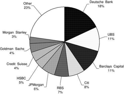
When one considers that many of the remaining banks in the business “white label” one or more of the top five's FX platforms to their own clients, we can see how dominant the top five players have actually become. Those banks that failed to recognize the change have been left behind, and the technological and infrastructure costs of rebuilding their businesses are now too prohibitive for most of them to contemplate re-entry into the top tier. Many have slipped into niche roles or have developed products that are designed to help their clients manage risk, as opposed to providing liquidity.
The FX market has seen the emergence of independent electronic trading platforms, such as EBS (ICAP Group), FXall, and HotspotFX, that provide liquidity to the market. Recently, these platforms have reported a growth in business-to-business transactions thereby bypassing the banks. In some instances this accounts for over 50 percent of the platform's turnover. Smaller niche providers, such as FrontierFX, have targeted the professional market, and this sector looks set to continue to grow.
One of the positive aspects of this revolution in the industry has been that foreign exchange, as a traded market, has become much more egalitarian in nature. The dissemination of news and information, that was formerly the province of the privileged few, is now available instantly over the Web. As a result, the major institutions now have little temporal advantage with respect to information. More importantly, there has been a dramatic fall in transaction costs in the industry in recent years. This has been driven primarily by the advent of electronic trading, which has encouraged competition and liquidity provision. But it has also coincided with the growth in speculative retail trading platforms that have allowed the smaller investor access to a market that was previously only available to the professional investor. The entry of these new participants in the sector has provided the market makers with new sources of liquidity and revenue.
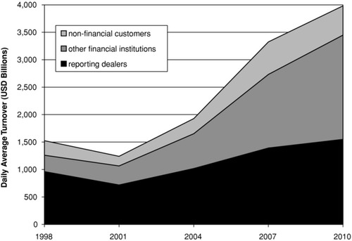
FX is now viewed as an “asset class” by many speculators and investors that had previously confined their investments to stocks and bonds. The dramatic increase in volatility in these traditional markets following the credit crisis has led investors to look at alternatives, and FX has been a significant beneficiary in terms of risk allocation and turnover. The increase in volume is clearly evident in Exhibit 16.2.
Exhibit 16.2 Global Foreign Exchange Market Turnover by Counterparty
Source: BIS Triennial Central Bank Survey of Foreign Exchange and Derivatives Market Activity, April 2010.
Perhaps the biggest contributor to growth in speculative FX trading has been in the area of systematic and algorithmic trading. A decade earlier, trading of this kind was seen as a minority activity and was mainly confined to a few hedge funds and sophisticated treasury operations. The majority of traders were discretionary, and what short-term trading there was remained mainly confined to proprietary trading within the banking industry.
One of the catalysts for this growth in systematic trading was the availability of accurate, reliable, and inexpensive high-frequency data. This allowed anyone who could handle a spreadsheet the opportunity to test and develop trading systems. Many saw this style of trading as an alternative to discretionary trading—which required a skill set that could only be acquired through years of trading experience. This increased availability of data coincided with a reduction in the cost of transacting in FX and with the growth of margin-based trading platforms offering multi-product electronic trading. The result was that many new speculators were attracted to the market.
One of the fastest areas of growth has come from commodity trading advisors (CTAs), quantitatively driven managed futures funds, and hedge funds that have adapted trading systems that had earlier been proven in equities and fixed income markets. Many of these funds have developed high or ultra–high frequency trading systems that now account for a significant percentage of daily turnover in the FX markets. These new entrants wish to trade electronically. Only those banks that had developed their own proprietary electronic trading systems were positioned to benefit from the business. The BIS triennial data (see Exhibit 16.2) has shown, for the first time, that the turnover from non-financial institutions now exceeds that of the banking sector for the first time.
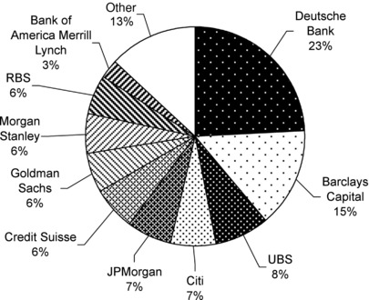
The Euromoney data in Exhibit 16.3 shows that leveraged funds make up a significant proportion of this sector, and the concentration of flow to banks servicing it is significant both in terms of profitability and information.
IS SYSTEMATIC TRADING JUST FOR GEEKS AND QUANTS?
Although some areas of systematic trading require a strong mathematical background, this is by no means true of the sector in general. Systematic trading can be as simple or as complex as one wants to make it. What systematic trading does provide is the opportunity to conduct detailed analysis of trading strategies and risk management. This is a fundamental and ongoing part of successful trading. Relying on a selective memory is, unfortunately, no substitute for cold facts.
All successful traders are systematic and disciplined in their approach to trading. The shelves of bookshops around the world are loaded with acres of books selling advice on how to become a successful trader. As many have found to their detriment, speculating successfully in any market requires more than the accumulation of these weighty tomes and blindly following someone else's “trading system.” Doing so will invariably result in trading losses or worse. This is because:
- Having not tested the strategy yourself over a suitable period of time, it is difficult to satisfy yourself that it actually works.
- Faith in the system will begin to erode during a significant drawdown (i.e., a period of losses), and there is a temptation to stop trading the strategy(s) and thereby lock in losses.
- There is the temptation to employ some discretionary overlay to the strategy that is untested, subjective, and driven by emotions.
However, if we look beyond the hyperbole surrounding these systems, we find that the common theme behind all successful trading approaches is a structured and disciplined application of the system in question. If fact, many experienced traders believe that it is the way a position is managed and not the position itself that is important in trading.
All traders employ approaches that make sense to them. These have generally been developed over a number of years and are the culmination of different experiences gained from trading in the market. Whatever system one uses, it is important that it be based on a rational analysis of the market or on some behavioral aspect of its participants. However, beyond that, there are as many ways to trade markets, as there are traders. It is helpful if the strategy can be tested in some way to validate the assumptions and the clearly defined rules that make it work. Many of the most successful traders employ this process religiously during every trade in order to keep subjective decisions to a minimum.
Becoming a successful trader is the process of developing a disciplined approach that works well over a significant period of time. If we accept that all successful traders are systematic to some significant degree, we need to examine how best to develop and employ a systematic approach to trading FX and to examine the benefits and limitations of such an approach. Although there is no substitute for actual experience, live trading can be a very expensive way to test ideas. Paper trading is a logical and less expensive substitute; but it still requires the benefit of time to observe and fine-tune the approach. On the downside, paper traders are prone to employ subjective ex post rationalizations.
Testing simple logical ideas and examining the outcomes can be a very rewarding and informative process. It has been the bedrock of modern scientific thinking for the past 300 years and has its role to play in trading markets. All that is needed initially is a reliable data set for the market traded and some basic spreadsheet skills. Although many traders associate trading success with complex systems, the opposite is more often true. This chapter is not intended to provide the reader with a “how to guide” to model building. There are a plethora of books available on that subject. We are more concerned here with describing the benefits, as well as the limitations, of testing and employing systematic trading models. Importantly, we are not advocating a complete change for those of you who employ a discretionary approach. Although some systematic zealots would disagree, being systematic does not preclude the use of discretion or judgment in decision making. However we would suggest that this is best employed in a non-emotive and, if possible, predetermined way to take into account extraordinary events.
One further word of caution with regard to testing in financial markets: It is helpful to remember that markets are essentially social and not physical systems and are made up of all the participants in the market at any one time. All social systems are subject to sudden behavioral changes. Such behavioral changes can be at odds with the assumptions we made when we were developing our model. As recent events have shown us, markets can behave in a chaotic manner, and models tend to perform poorly in such environments.
WHAT CAN SYSTEMATIC TRADING ANALYSIS DO FOR ME?
You learn most from your mistakes, not your successes. You have to handle getting your butt kicked and learn from it.
Paul Tudor Jones
Learning from your mistakes is a good place to start, and one of the real benefits afforded to systematic traders is that they can analyze their trading history in some detail. It is very difficult to avoid the effects of selective memory when conducting an objective appraisal of trading success. For the discretionary trader, this is also a good place to start. Many successful traders keep a detailed record of all of their trades including not only the entry and exit points, but also the rationale behind each trade. The more information we have, the better the analysis.
What can analyzing a trading history reveal?
1. Your ratio of winning and losing trades:
- Winning and losing sequences go on longer than you would expect.
- This is especially true of trend traders.
2. The average size of your wins and losses (as a percentage of the value of the position):
- An average of 0.550 percent on wins and –0.45 percent on losses over time would be excellent.
3. Winning and losing trades by strategy/market:
- There is a tendency to trade markets we are most comfortable with. This is not always the most profitable use of resources.
4. The average holding period of your trades:
- There is a direct relationship between volatility and time. The longer you hold a trade, the bigger the P&L swings.
Systematically analyzing a trading history can reveal a great deal about the trader and his or her approach. The more information we have the more detailed and useful the analysis. Top athletes analyze their game on an ongoing basis, trying to identify areas of strength and weakness. The trader should be no different.
ADVANTAGES AND LIMITATIONS OF SYSTEMATIC TRADING
For many traders, distilling their trading approach into a couple of simple rules can be a difficult process that they do not wish to attempt. However, doing so is a worthwhile activity: The cathartic process of defining a trading approach can be extremely revealing to both systematic and discretionary traders alike. Patterns that we believe we have discerned from the market are often illusory.
Advantages of a Systematic Approach
Removing the emotion from trading decisions: Trading is very emotional, as anyone who has experienced the euphoria of having a position go right will testify. Unfortunately, the flip side of that experience is the “fight or flight” reaction that is triggered when you are losing money. This type of reaction is very useful when running away from predators, but often counterproductive in a market context. Research has shown that this type of reaction shuts down the parts of the brain responsible for logic and reasoning. Losing money is an inescapable part of trading, so the emotional response to “escape” from a losing position can be very harmful. Having a trading system means that one can dispassionately make decisions in advance about how positions are to be managed. In essence, it can override the instinctive and counterproductive response in those fight or flight moments.
In-built trading discipline: One thing most top traders will agree on is that discipline is vital to trading success. Adopting a disciplined approach is hard work. One advantage of creating systems is that they can enforce discipline in the form of stop-loss levels and prompt entry to trades (the least obvious trades are sometimes the most profitable).
It is testable: This is the biggest single advantage. Market literature and accumulated folklore are overflowing with indicators, technical levels, fundamental drivers, candlestick patterns, and what have you, all claiming to tell you whether the market is going up or down. The majority of these will fail to live up to their promise. As humanity learned some time ago, the best way to distinguish between superstition and reality is to test.
Of course, even gut feeling trading can be tested. With a long enough history of trades, you can work out when your gut feel has worked and when it hasn’t. However, if someone comes to you with a new trading idea today, how can you evaluate it? If the idea can be written down with enough clarity to form a series of rules, it can be tested—in fact, just seeing if it can be stated clearly in this way is a good test of whether it has any merit.
Although it is not a substitute for an actual trading history, testing is an extremely valuable way to see if the claimed approach works. Essentially, if you have market data for a sufficiently long period, say 10 years, and a trading idea that can be stated as a set of rules, you can create an artificial “trading history” complete with trade entries, exits, and P&L that would have been experienced by someone mechanically following your rules during those years. This approach is called backtesting, and we will say more about it later.
The emphasis on testing might strike some as unnecessary. If a pattern in the market is obvious to the eye, why bother? The answer was given by physicist Richard Feynman, albeit in a different context:
The first principle is that you must not fool yourself, and you are the easiest person to fool.1
The human mind is very good at pattern-matching, but the penalty for that is that we can get a lot of false positives. Take the example of pareidolia, where human faces are seen in a variety of entirely natural objects such as the surface of the moon or burnt tortillas. We are very good at recognizing faces—so good that we will even see them where they do not exist. Another example is the canals on Mars, which were extensively mapped in the nineteenth century, until an experiment in 1903 showed them to be an optical illusion caused by our tendency to “join the dots” of craters when seeing a blurry image. The only defense against fooling ourselves in this way is to test in a non-emotional and non-subjective manner.
Why Systematic Trading Is Not a Magic Bullet
It may seem perverse to include a section on the drawbacks and problems of systematic trading, but like most powerful techniques it has its dangers, and is easy to misuse. The trouble is that many of the misuses of trading systems will not be immediately apparent: the tested performance will look very good, and no problems come to light until the system is traded live.
The truth is that a lot more trading ideas look as though they work than do actually work. Backtesting is great for instilling confidence that an idea is genuine, and, armed with a simulated “equity curve,” it is easy to think that you have come up with a foolproof moneymaking machine. An equity curve depicts the cumulative percentage change in the trader's equity over time as a consequence of trading. Good-looking equity curves are both beguiling and remarkably easy to produce. Unfortunately, although all good ideas backtest well, a lot of bad ideas do too, and it is a truism of systematic trading that backtests invariably look better than real trading performance. It is a fallacy to think that this can be overcome by just making the backtested performance worse in some way, such as by reducing the return. For a bad model the actual trading results can be unrecognizable from the backtested equity curve. Why is this?
Fitting the Noise, Not the Data
Market data is noisy—it contains a lot of “random” ups and downs, along with the signal that your system is trying to extract and profit from (of course, exactly what is “signal” and what is “noise” depends on what the system is, and its timescale). What you would like the test to do is tell you whether the signal your system is trying to exploit is a real recurring pattern in the historical data. However, the test is actually answering the question “Is there any way at all I can make this work?” It is very easy for random, unrepeatable price action to accidentally give positive P&L, and any attempt to search for the right parameters to use will highlight these “lucky” accidents. This may seem unlikely, but bear in mind the Pareto principle that 80 percent of your P&L comes from 20 percent of your trades. Good luck has a lot more impact than you might expect.
Over-Optimization
In backtesting, it is very common to vary the system parameters to find the “best” value. A parameter is any input that you can vary. For example, in a simple moving average, the number of days over which you “look-back” is a parameter. If the system is traded once per day, then the time of day you execute is also a parameter. The more complex a trading system is, the more parameters it will require, and the more tests you have to do to find the best values for those parameters. For example, if there is only one parameter, then you may wish to try 20 different values for that parameter to see which gives the best results. If you have two parameters and you would like to try 20 possible values for each, then you will be searching through 20 × 20 = 400 different combinations of parameter values. For three parameters it will be 8,000. It is relatively simple to get a computer to search all values of these parameters, but the more tests you do, the more likely you are to find “something” where nothing actually exists (this is known in statistics as the “multiple comparisons problem”). By the time you get to four parameters, even random trading signals can generate an excellent equity curve with double-digit returns and a good risk/return ratio—all purely by chance. This is illustrated in Exhibit 16.4.
Exhibit 16.4 The Effect of Change: Random Trading in EUR–USD (the best result of 160,000 equity curves)
For any given trading algorithm requiring parameter selection (and all algorithms will require some form of parameter selection), you will end up with an equity curve that looks as good as it can possibly look over the historic period used to develop the model.
Parameter Choice
When trading a model out-of-sample—that is, into the unknown future, not with the same data you used to determine the parameters—it is very unlikely that the parameters chosen will be the perfect parameters for the new period. The best case is that they are still good. The worst case is that they are completely inappropriate. It may be that the trading rules would still work, but only with a different set of parameters that you could not possibly have chosen in advance. This is the difference between a model that is robust and one that is brittle. Ultimately, a system that has parameters that are impossible to specify in advance is useless. It will always backtest well, but never perform well out-of-sample.
Past as Prologue—Or Not
Even if you have found a genuine effect in your backtest, the market is ever-evolving. It may be that the model trades successfully for some time out-of-sample, but a systemic shock or other change in the way the market trades could eliminate the anomaly that you were relying on. It is likely that all models have “lifetimes.” What separates a robust approach from a brittle one is the length of time for which the parameters or algorithm can be relied upon for successful trading.
Position Management
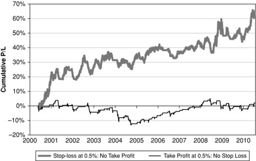
Even good trading signals are no substitute for good trading discipline and position management. It might be assumed that the directional signals generated are of primary importance, and that position management is only a second-order effect, but this is unlikely to be true. Consider the following equity curves depicted in Exhibit 16.5. These were generated from a momentum-based trend-following model using two different exit rules. In one case, the model employed a rule requiring that profits be taken if, and when, a specified positive P&L level was reached. This version did not employ a stop-loss, so losses could run. In the other case, a stop-loss rule was employed at a loss level that mirrored the P&L level of the first rule. This version did not take profits at a target level so profits could run. It is worth noting that taking profit early and running losses is characteristic of undisciplined, emotional trading behavior—our brains are wired to see stop-losses as a “punishment” and take-profits as a “reward,” so we tend to seek the latter and avoid the former. Backtesting shows how damaging this is to performance!
Exhibit 16.5 Effect of Position Management (EUR–USD trend trading)
How Can These Mistakes Be Avoided?
It is impossible to say with certainty that a model is robust, but it is possible to weed out a lot of candidates by rigorous testing. It is very difficult to walk away from a model that looks profitable on paper, but this can often be the wisest course of action. The important thing to be wary of is confirmation bias, which is the tendency to seek out supportive evidence and dismiss the negative. You must be your own worst critic. You must actively seek out evidence that your system does not work and identify the failure modes that could cause it to lose money. Unless you have seen how badly it can perform, you have no grounds for confidence—and remember, backtesting will systematically sweep the flaws under the carpet. Testing on other data sources is not always possible, but is a good idea, as it guards against overfitting to random fluctuations in the original data set.
The question of how sensitive the model is to changes in its parameters is very important (see following). A useful warning sign is that all its profit has come from one or two short periods in history. Lastly, and very importantly, is the model code itself correct? That is, if a model is a candidate for live trading, it is wise to have it independently rebuilt from scratch using only a specification of the algorithm.
WHAT IS NECESSARY FOR A SYSTEM TO WORK?
Any list such as this can only ever be “necessary, but not sufficient.” Having said that, any model that has the following is more likely to be valid:
A clearly defined rationale: This should be explicitly decided and preferably written down prior to constructing the system itself. Every model has an underlying market behavior that it is trying to exploit. The best models express this clearly and simply. Some corollaries to this are:
- Don't tinker: It has been said that exceptions make bad laws, and this is also true of rule-based trading. Putting multiple exceptions into your code just overfits history, and leads to a multitude of parameters, which will guarantee a good-looking, but meaningless, equity curve.
- Don't post-rationalize: Explanations of model behavior after it has produced a good equity curve always sound convincing, but are rarely useful. It should be borne in mind that your system's performance cannot be evidence in favor of an ex post rationalization as to why it works. If your post-rationalization can be tested, you can determine if it is valid; if not, it's a nice-sounding explanation that may make for good marketing copy, but nothing more.
Entry and exit conditions: This may sound obvious, but it is surprising how many well known “trading systems” are out there that consist entirely of entry signals. Such a “system” is in fact only half a system: it cannot be tested because the exit signals are crucial in determining its profitability or otherwise. Systems that trade continuously and reverse position are fine, but otherwise the exit signals must be part of the specification.
A small number of parameters: These must be specifiable with some confidence. We have already established that large numbers of parameters make good results much less significant. It is also likely that in a many-parameter model, the parameters will not be independent; that is, the values of one parameter will depend on the values of the other parameters. This means that rather than getting the values of the individual parameters right independently, you must get the combination exactly right—a much harder task.
To some extent this is inevitable, but it can also signal that your parameters perform a similar or overlapping function in your trading system, and that the rules should be simplified to reduce the two overlapping parameters to a single one. Note that this simplification will always make the backtest look worse! Ideally you should have a feel for what the parameters should be prior to searching, thus transforming a data-mining exercise akin to flipping a coin many times into a real test of whether reasonable parameters perform acceptably. It is much easier if your parameters have meaning, that is, correspond to measurable things like market volatility or an average day's move.
WHAT CAN I REASONABLY EXPECT?
Risk/Return Ratio
The trade-off between the risk and the return associated with a strategy is commonly measured via the Sharpe ratio. The Sharpe ratio is the annualized excess return of a strategy divided by its annualized volatility (i.e., risk).2 By excess return we mean that we deduct the risk-free rate of interest from the strategy return. Because return is in the numerator and risk is in the denominator, the higher the Sharpe ratio, the better. The major driver of volatility for a system that can trade no more than once a day is the underlying market volatility. So for a market volatility of 10 percent, a system with a Sharpe ratio of 1.0 would have an annualized excess return of 10 percent. Backtests can easily give Sharpe ratios of 2.0 or more, but, as noted earlier, backtests always exaggerate performance. Over the long-term, a Sharpe of 1.0 is good, and 0.5 is about average. Quoting Sharpe ratios for periods shorter than one year gives nonsensical results and should be avoided. Note that the preceding figures exclude ultra–high frequency (UHF) trading systems: such systems trade much more frequently, and can have very high Sharpe ratios. For such systems, the true risk is not market volatility leading to P&L fluctuations, but systemic breakdown of the trading methodology, which typically leads to sudden unprecedented large losses. The equity curve for UHF trading generally does not give a good representation of the real risk, which can be hard to quantify.
Maximum Drawdown
Maximum drawdown (MDD) is a measure of how far the portfolio's cumulative P&L has fallen below a previous high water mark. MDD is measured as the difference between the highest equity attained and the subsequent low point, and calculated on a daily basis. It is a popular measure because it is perceived by many as a “worst-case-loss scenario,” that is, the experience of the unluckiest investor in a program who joins immediately before the largest sustained loss. In practice, MDDs measured from backtests tend to be optimistic. Backtests are always rose-tinted, and large drawdowns are necessarily rare by virtue of being extreme events. Maximum drawdowns can only increase with increasing length of track record: a short track record with a low MDD merely means that nothing has gone wrong yet. MDD scales as volatility, in that a model with a 20-volatility rating (possibly due to trading at greater leverage) will have twice the expected MDD of a 10-volatility model. But, in the high volatility case, the MDD is more uncertain—the worst-case could be a lot worse in the high volatility model. The ratio of return to MDD is called the Calmar ratio3 and is sometimes reported along with the MDD. Over a realistic timeframe, a Calmar ratio of 1.0 is considered good, and anything higher probably understates the MDD risk or overstates the return.
Win Ratio
The win:loss trade ratio is highly strategy-dependent, but if we consider it on a per-day basis there is a clear, linear relationship with the Sharpe ratio. This can be tested with a dummy “trading model” that has daily signals with a user-specified win ratio, using real market data. Using results from this model, it can be seen that a Sharpe of 1.0 corresponds to a daily win:lose ratio of 54:46 (assuming you're not getting all the big days wrong). By contrast, a win:lose ratio of 70:30 would give a Sharpe of 5, which is very unrealistic unless trading in an ultra–high frequency system.
Industry Comparisons
There are various hedge fund indices available against which a trading strategy's performance may be benchmarked. Obviously, it only makes sense to do this with out-of-sample performance results as opposed to backtest performance results. Regrettably, there are some problems endemic in the industry when it comes to reporting results. The index may contain backtested “performance” figures, as performance is usually self-certified by the data providers (i.e., the hedge fund managers) themselves. The differences between backtest performance and real trading performance may be ignored in the published index. It is also common practice to remove the track record of funds that have ceased trading (usually due to unsatisfactory performance) from the entire index, historical and future. This creates a huge survivor bias in the reporting: it is perfectly possible to get a good-looking index from random data if the losing results can be excluded! This survivor bias (often called survivorship bias) can have a huge effect, and has led some industry figures to speculate whether the hedge fund sector as a whole may have negligible returns net of fees if these effects were corrected for.4
USES OF SYSTEMATIC TRADING METHODS
A trading model gives a directional signal for a particular market. This may incorporate strength of signal (anywhere between 0 and 100 percent) or be digital in nature: long, short, or neutral. Although trading signals are necessary for any systematic trading program, we need to consider how these signals are used in practice. We will then look at the two main applications of systematic trading: speculative trading and hedging programs.
Construction of a Systematic Trading Portfolio
In stock trading, a portfolio is a collection of stocks, which may be held in different quantities, which are thought of as a unit in the expectation of a reduction in volatility and improved risk/reward ratio when compared to trading single stocks. This principle also applies to systematic FX trading. But, as the number of relevant currency pairs is small in number compared to the number of publicly traded stocks, diversification is achieved by trading different models, as well as different currency pairs.
In order for this to be of any benefit, the models must offer returns with a low correlation. We can summarize the different forms of diversification as follows:
1. Diversification across markets: This form of diversification is the most similar to the stock analogy. It aims to produce uncorrelated returns by trading many different currency pairs. If different currencies are driven by different underlying factors, the patterns and price action exhibited by different currency pairs will have little to do with each other, and thus the same model traded in different markets will produce a different pattern of returns. This is most pronounced when the currency pairs do not share a currency in common. For example, although EUR–USD and GBP–USD will offer some diversification, they share exposure to USD factors. It would be reasonable to assume that EUR–JPY and GBP–USD would have lower correlation.
2. Diversification across models: Different trading models earn their returns based on different market behaviors. The simplest example is trend following, which aims to profit from sustained directional moves. On the other hand, mean reversion trading aims to profit from the opposite type of behavior, where a move is reversed rather than extended. These two systems would be expected to have a very low, or even negative, correlation, leading to good portfolio effect.
3. Diversification across time-scales: Surprisingly, running two similar models in the same currency pair can yield diversification if one model is long-term and the other is short-term. In the example of two trend-followers, one might aim to profit from moves in the one-week time horizon, whereas the other may be looking for longer term-moves of a month or more. Although they will have the same position in the face of a long-term trend, their signals will offset each other for a significant proportion of the time, especially when the signal is not clear.
Unfortunately, portfolios designed with diversification in mind can fail to deliver the expected benefits. Some of the most important factors affecting them are:
Exhibit 16.6 EUR–JPY and AUD–USD Spot
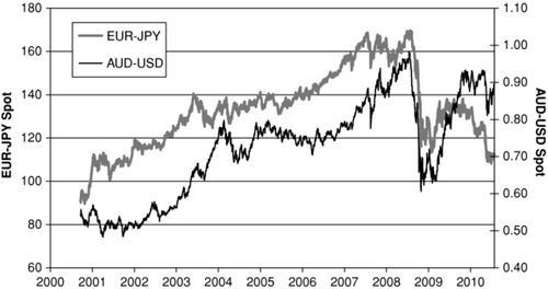
1. Illusion of diversification: It may appear that EUR–JPY has nothing to do with AUD–USD, but since September 2008, their average 1-month rolling correlation has been 0.69, with a peak of 0.97. More importantly from a trader's perspective, the direction and timing of trends looks very similar when viewed on a chart. See Exhibit 16.6. If the market currently views both these currency pairs as “risk trades,” an outbreak of risk-aversion would affect both of them in a similar fashion. This is especially true for U.S. dollar–based currency pairs, where the dollar can easily be the driving factor, and the expected diversification largely evaporates. It should be remembered that in a strongly directional market, there is only one way to make money, and those models whose signals line up on the right side of the market are doing their jobs correctly—but won't be adding diversification.
2. Dilution of returns: It turns out that it is remarkably easy to diversify away returns as well as risk. For example, imagine trading both a trend-following system and a mean-reversion system at the same time to gain diversification. If the two models have similar time-scales, it is highly likely that what one model makes, the other one will lose—excellent diversification, but no profit! It is normally argued that if the expected return from each model is positive, the expected outcome will be positive, but this overlooks the fact that the models are not independent. In a given year, a strongly trending market is very likely to give poor, or even negative, returns for the mean-reverter, and likewise a market full of reversals will cause the trend-follower to lose money. This can easily mean that the “average case” becomes the best case, and the actual returns are far smaller than envisaged.
Exhibit 16.7 EUR–JPY and AUD–USD (Correlation versus Size of Daily Move)
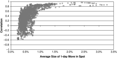
3. Correlation increases during market shocks: Even currency pairs that are uncorrelated under normal market conditions can have the same reaction to an extreme event. Global news events can have traders “fleeing to quality,” with the result that any currency seen as overly risky suffers a move in the same direction (see Exhibit 16.7). These shock moves are typically against the prevailing trend (especially if the trend is in favor of the carry trade, which is almost always vulnerable to these events). Thus, all models that are currently profitable are liable to suffer a drastic reversal of fortune at the same time. These sorts of breakdowns in historic correlation are typically accompanied by market moves in the “fat tails regions.” This can lead to a double-whammy effect that can put incautious traders out of business. The difference between the average case and the worst case for a large portfolio tends to be substantial, and shock events can make the worst case much more likely than a naïve treatment of risk would suppose.
Considerations in Portfolio Design
So, what makes for a well-diversified, robust portfolio? A great deal has been written on this issue including some of the most important financial theory—most notably what is now called Modern Portfolio Theory, which we will discuss shortly. For the moment, however, there are some common-sense considerations that must be applied to any allocation decision. The question is, in essence, extremely simple: “What amounts should I trade in each of my trading models in order to maximize my projected return for a given level of risk?”
The first thing to note is that, in order to achieve a reduction in volatility compared to trading a single model, it is necessary to have meaningful amounts trading in more than one model. Diversification happens when the P&L from one set of models partially offsets the P&L from another set. If the allocations are such that a single model, or subset of models, has an overwhelming allocation of capital, then not much offset is possible and little risk reduction is achieved.
Conclusion: Portfolio weights must be roughly evenly balanced for maximum risk reduction through diversification.
The second thing to note is that not all models and not all markets are equal. Some are more risky than others. Volatility is the standard measure of risk, and can be thought of as a measure of the average size of move that can be expected. Double the volatility and you would expect market moves of twice the size. As the events of 2008 and beyond showed, the assumption that foreign exchange market volatility is roughly constant at 10 percent is invalid, even if some currency pairs have now re-entered that regime. The credit crunch caused some markets to triple or even quadruple their volatilities in under a month. This dramatic increase in volatility, however, was not experienced to the same extent by every currency pair, causing large risk disparities.
Conclusion: Portfolio weights must take account of risk, and must be periodically re-balanced to allow for the changing risk profile of different markets.
It is worth noting, in passing, that varying risk levels cause a problem in the overall level of risk in the portfolio, as well as the relative weights of individual models. This relates to the total position size, or leverage, of the portfolio, and will be addressed later.
Two Portfolio Design Approaches
Modern Portfolio Theory (MPT) Approach
Despite its name, MPT dates from 1952.5 The central concept is that knowledge of how the various portfolio components correlate (represented by a correlation matrix), together with their expected returns (usually derived from historical performance), allows one to calculate the optimal weightings that will give the best answer to the question posed earlier; that is, “What weighting scheme will maximize return for a given level of risk?” Different levels of specified risk will be associated with different levels of maximum expected return. And associated with each of these risk/return points is some corresponding portfolio composition (i.e., weighting scheme). Collectively, these risk/return points make up the so-called efficient frontier.
MPT is mathematically elegant and provides well-defined solutions to the problem of portfolio weights. But any model is only as good as its assumptions. Critical to MPT is the assumption that correlations are stable and that expected returns are estimable. So, one needs to ask “How stable are the correlations between the different models, and how well can we estimate the expected returns?” Correlation is a famously slippery concept. By changing the historical period used in the calculation, one can derive widely differing correlation coefficients. This is illustrated for the EUR–GBP and USD–JPY currency pairs in the Exhibit 16.8.
Exhibit 16.8 EUR–GBP and USD–JPY 3-Month Correlation (Weekly Data)
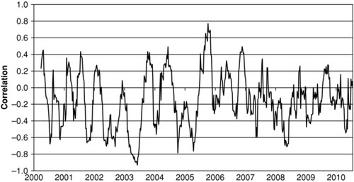
MPT results are sensitive to changes in the correlation inputs. Given the variability in historical correlations, it is no surprise that future correlations may differ widely from those expected. The second problem is in estimating historical returns. Although this is simpler, it still assumes that the future P&L of a model is well represented by the average P&L over a long period. In practice, even a well-performing model can have poor years, and similarly a poor-performing model may have some exceptionally good years. This means that the P&L for any given model with a realistic risk/return profile may differ greatly from the average case, which in turn means that the “optimal” portfolio weights employed may be far from optimal in any given year.
The net result of these two uncertainties, smuggled into the assumptions of MPT, is that there is a great deal of uncertainty in the optimized portfolio weights it generates, which lays it open to charges of over-optimization. There is also the problem that, for any given portfolio, the component weightings may be far from equal simply because of a correlation between two trading models that arose by chance (sometimes called “spurious correlation”). As soon as this chance effect breaks down, the weights that were calculated become invalid. The results of a MPT optimization are liable, therefore, to be brittle rather than robust. For this reason, the process should be used with caution, and heavily constrained to ensure a sensible answer.
“Old School” Approach
This approach eschews any form of optimized solution in favor of the simple maxim of equal weights for everything. Although this may seem primitive, it has a number of advantages. As the weights aren't optimized, there is no danger of over-optimization based on history that may not be repeated. Very few assumptions are made about relative performance levels, and the main challenge is setting the overall leverage of the portfolio.
The problems associated with this approach come from the failure of the assumption that all models and markets are created equal. For example, a model trading GBP–USD may have half the P&L volatility of the same model trading GBP–JPY, but this approach would weight them the same. A modification of this approach, weighting things equally by risk, rather than by face amount, goes a long way toward solving this problem.
It is worth noting that employing conservative assumptions for correlation and knowledge of future returns in an MPT analysis often gives results very similar to this “Old School” approach.
Leverage and Margin Trading
Having decided on the relative amounts (i.e., weightings) that will be applied in a portfolio of trading models, one must next decide how much to allocate to the portfolio in total. This is normally decided with reference to either an investment amount or a risk budget—or, more commonly, a combination of both.
In a traditional hedge fund structure, the investment amount is defined as the capital (including reinvestment) that the investors have placed in the fund structure. Here, the leverage is defined as the ratio of total position size to that investment amount. If the two are the same, the fund is said to be unleveraged (or running at one-times leverage). Running at higher levels of leverage implies a larger total position size, engendering both more volatility and higher potential return.
Systematic trading is commonly done via margin trading—in fact, some of the first systematic traders were the so-called commodity trading advisors (CTAs), which traded managed futures funds (sometimes called commodity pools) using on-exchange margin trading. Margin trading has the advantage that you do not have to deposit the whole investment amount on day one (which can be very cash inefficient). Instead, the margin account must be sufficiently funded to cover all projected trading losses—an amount that can be as little as 10 percent of the equivalent investment amount. The notion of an “investment amount” is largely hypothetical in margin trading, which can make it difficult to compare returns between managed futures funds and conventional funds. Sometimes margin traders will quote returns as a percentage of margin, which can result in some very large and misleading percentage figures for return and risk. The only valid way to compare different funds is to compare return per unit risk, which is commonly done by the Sharpe ratio.
The Sharpe ratio is the most commonly used risk-adjusted return measure. It is nearly universally employed in the hedge fund and CTA worlds. As previously noted, it is defined as the annualized excess return divided by the annualized volatility of those returns, normally measured from daily return data. To obtain the excess return, the risk-free rate on any funds deposited must be deducted from the trader's return.6 As the Sharpe ratio is annualized, the minimum acceptable period over which to calculate it would be one year. Calculating the Sharpe ratio over a short period of good performance will result in a misleadingly high ratio that may bear little relationship to longer-term performance.
Risk targeting is commonly done using either maximum drawdown (discussed earlier) or volatility measures. Any margin trading system must ensure that sufficient margin is available to cover a maximum drawdown event. The problem with MDD as a risk measure is that it is often taken as a “maximum loss limit,” whereas in fact it can only increase over time. MDD events are by definition rare, so relying on them as a true indicator of the risk to which a portfolio is exposed is dangerous. Volatility is a more reliable risk measure, although it does not have the direct relationship to margin that makes MDD popular. Funds are commonly described by either their volatility target or the leverage they employ. As volatility can be highly variable, this targeting can only be approximated using any of a number of possible techniques to estimate current and future portfolio volatility.
Currency Alpha and Beta
The Capital Asset Pricing Model (CAPM) was introduced over the period 1961–1966, and classified stock returns as alpha and beta.7 The beta return of a stock is the portion of its return that is explained by movements in the market index or by the market as a whole. A stock with a beta of 1 would be expected to produce returns equal, on average, to those of the market as a whole. Beta, in this context, is often said to represent the “systemic” risk exposure of the stock. The alpha is the portion of the stock's return that is not explained by the market as a whole, and therefore represents “pure” or uncorrelated return.
The application of alpha and beta to currency markets is not immediately obvious. There is no “market” as a whole that can be invested in, and every purchase of a currency is ipso facto the sale of a different currency. However, from the perspective of a stock investor, the returns from currency trading would represent “pure alpha,” as they have been largely, or even entirely, uncorrelated to the stock market (i.e., zero beta). It has thus become customary to refer to currency trading returns as providing “currency alpha.”
In the last few years, it has been increasingly common to hear currency referred to as an “asset class.” To quote the Yale Endowment in 2005, “The definition of an asset class is quite subjective, requiring precise distinctions where none exist.” This sort of language was first adopted by large investment banks seeking to sell foreign exchange products to conventional asset managers, so it may be suspected that this was an attempt to co-opt the language of asset management to sell trading products that asset managers might not otherwise consider within their remit. The truth is that foreign exchange contracts and stocks have both similarities and differences. The similarities chiefly relate to the fact that they can both be traded in a liquid market. It may be more accurate to say that foreign exchange is a risk class rather than an asset class: It is an arena in which market risk may be taken in order to earn an expected return. The difference between this and a conventional stock market is that “buy and hold” in FX is not a strategy with which anyone should expect to make money long term.
Some practitioners have taken the analogy between FX trading returns and conventional CAPM modeling further. It is not uncommon now to see “currency beta” products offered, some of which have been securitized. These define beta as the systematic exposure to artificial indices associated with different styles of trading. By using mathematical techniques, such as multivariate regression, and fitting them to various industry performance benchmarks, they calculate standard strategies that represent “pure” trend trading, carry trading, and mean reversion. An individual manager's performance may be compared to the performance of these strategies and a beta calculated in the same way that a stock beta is calculated with reference to the stock index's performance.
These “pure beta” strategies are now offered as trading products by a number of leading institutions. Whether such an approach has any validity depends largely on the way in which the products are used. Many asset managers seeking to diversify into the hedge fund arena seek to gain exposure to different styles of trading, but are obliged, by absence of choice, to invest in a “fund of funds” to do so. The disadvantages of this approach are many, including the potential for style drift and a double layer of performance fees. If all that is desired is to gain exposure to a typical pattern of, say, trend trading, then a “pure trend beta” product offers a cheaper and more transparent alternative—free from problems of individual manager misjudgment or style drift. If the individual manager wishes to buy and sell “trend” as a commodity (in much the same way that the VIX secondary market allows people to buy and sell volatility), then this is an ideal vehicle. If, on the other hand, the asset manager wishes to buy and hold a portfolio of beta strategies, the analogy to the stock market collapses, as there is a paucity of evidence that this approach will produce positive returns over the long term. Viewed in this way, “currency beta” strategies are just simplistic trading systems designed to look like everyone else rather than to make money.
Systematic Hedging
Hedging systematically has a long history. For many companies, it is common practice to cover their exposures using a program of trades, such as rolling forward cover or a strip of options. Although these are systematic, they are passive and in no way attempt to follow or react to the market, and therefore fall outside our purposes in this chapter.
However, a more active approach to hedging has been followed by some companies and financial institutions. In the same way that a speculator takes a view on the market and goes long or short to express that view, a hedger may increase or decrease a hedge to express the same view. The actions will be different depending on whether the underlying exposure is short or long for the currency pair in question, but the signals can be identical. The hedger is much more constrained than the trader: in order to qualify as hedging, the positions taken must always be against the underlying position, and cannot be a greater size than it. Also, the hedger does not have the freedom to specify which markets they wish to trade, but must only take positions in those markets in which the institution has exposure.
Example of Hedging Using Directional Signals
Imagine now Company A, which is domiciled in the United States and has net assets in Germany worth EUR 100m. In order to hedge its balance sheet exposure, the company's management decides to sell EUR forward versus the USD. They start by placing a forward hedge (the “constant cover”) for half the amount, that is, EUR 50m. The remaining EUR 50m is traded according to a systematic long-term directional program.
Suppose now that the system (i.e., directional program) generates a long signal. This would be in favor of the underlying exposure. The EUR 50m associated with the trading system is bought, offsetting the 50 percent constant cover hedge. The net hedge amount is therefore zero, and the company benefits in full from any appreciation in the EUR.
Alternatively, suppose that the system generates a short signal. This would be against the underlying exposure. Then the actively-traded EUR 50m is sold, adding to the forward hedge that is already in place, thereby hedging 100 percent of the underlying exposure. Company A is now fully protected from any weakening of the EUR.
Finally, suppose the system generates a neutral signal, implying no opinion on the direction of the EUR. Then the actively-traded part of the hedge is neutralized, leaving just the EUR 50m constant cover. The company is now partially hedged and will experience half the benefit or loss of any movement in EUR-USD.
Note that, in all of these cases, the actions taken with respect to the active portion of the hedge are identical to the actions that would be taken by a speculator trading EUR-USD with a EUR 50m position size. Thus, any speculative system generating trading signals may also be used for the purpose of hedging, although for practical reasons very high-frequency systems are generally unsuitable. As a side note, I would point out that, in some countries, adding a speculative component to a hedging program might result in the loss of the right to use hedge accounting, and this can have implications for the volatility of P&L. We will return to this point later.
Benchmarking and Risk Appetite
Depending on a company's risk tolerance level, sometimes called its “risk appetite,” several variations on hedging with the directional signals theme are possible. The risk appetite determines the company's “default hedge position,” which can be thought of as how much of their exposure they would hedge if they had no view on the direction of the relevant currency (i.e., the constant cover). In our prior example, the constant cover was 50 percent of the exposure, and it could vary from 0 percent to 100 percent depending on the directional system's indications. Now consider a company that has very little risk appetite and employs a constant cover of 90 percent, allowing itself a downward departure of only 10 percent when its directional system indicates the EUR will rise, but never going beyond its maximum cover of 100 percent when it thinks the EUR will fall. Thus, for the same size exposure as in our prior example, the company's hedge would vary from EUR 100m to EUR 80m, but would never go below EUR 80m.
Of course a company's constant cover could be anywhere between 100 percent (an entirely passive hedge) and 0 percent (entirely unhedged). For example, it might be 75 percent. In this case, with a similar exposure to the company above, management might wish to hedge EUR 75m as constant cover, and actively trade the remaining EUR 25m. This would result in a maximum hedge ratio of 100 percent as in the previous example, but a minimum hedge ratio of 50 percent. In this case, even when the signal is long, the company is still partially hedged. Although this may lead to hedge losses (if the signal is correct!), the P&L volatility and risk are constrained. It would also be possible to revert to a 100 percent hedge given a neutral signal, biasing the system further in favor of the full hedge. As this approach is fully hedged by default, and risk is measured as the deviation from that position, so Company A would be said to have a “fully-hedged benchmark.”
Importantly, the cash requirements associated with hedging can be substantial and may not correspond to actual receivables—as in the case of balance sheet hedging in the examples above. To avoid excessive P&L volatility and to preserve competitiveness against unhedged competitors, a company might choose an unhedged benchmark. This is the inverse of the above: by adopting, for example, a EUR 25m constant cover and actively trading EUR 25m, the maximum hedge ratio is 50 percent, and the minimum zero. It should be noted that the active portion of the hedging program is unchanged in this example from the fully hedged case: all that has changed is the magnitude of the constant cover hedge.
A balanced (symmetric) benchmark is also possible and would correspond to the EUR 50m constant cover hedge in the original example. However, there is nothing obliging Company A to actively trade the entire remainder. It would be possible to trade only 25m actively, giving a maximum hedge of 75 percent and a minimum of 25 percent.
In all of the above cases, the size of the actively traded portion defines the size of the deviations from the benchmark: in the symmetric case, by +/− the amount, and in the fully-hedged–unhedged cases, by twice the amount. The size of the active portion, therefore, should be related to the company's risk appetite—risk here being defined as deviation from the benchmark. In the limiting lower case (no active trading), this then defaults to being the passive benchmark strategy. The upper limit is as given in the original example, with maximum and minimum hedge ratios of 100 percent and zero.
Currency Overlay
Currency overlay is the outsourcing of currency risk management. A “risk discovery” exercise is performed to identify and quantify the nature of a company or institution's exposures. After the benchmark and risk appetite of the client has been determined, the overlay company trades the hedging program on behalf of the client, usually by a margin account/power of attorney arrangement similar to an investment management agreement for a CTA. The manager is normally incentivized by a flat fee. Performance fees are only appropriate in the case of a balanced benchmark, as otherwise the manager is penalized for reverting to the benchmark position, even when it is in the client's best interest. In any case, performance fees represent an incentive to overtrade.
Some overlay providers have been criticized for a “smoke and mirrors” approach, promising currency alpha plus a reduction in risk while ignoring the introduction of substantial tracking error, and sometimes overstating the performance of their actively traded component. The truth is that it is quite hard for overlay providers to add value. The choice of currency pair is not theirs to make, and it is rare for a trading system to work equally well in all currency pairs. They can only add value in one direction, unless the benchmark is symmetrical (overlay providers are much more in favor of this approach than most institutions), and the actively traded portion may only be a fraction of the total exposure to meet the client's risk appetite. Against this, some clients can display confusion as to the purpose of overlay: some may want to disguise a speculative program as a hedge, and be disappointed that the above constraints make it underperform.
Advantages and Disadvantages of Systematic Hedging
1. Quantify the “known unknowns”: A great advantage of systematic hedging is that expected performance and risk can be quantified in advance. Although there is still the unknown risk of systemic change leading to model failure, systematic trading allows future hedge performance to be forecast much better than with discretionary management.
2. Discipline: Best practice: With many companies and financial institutions employing consultants who demand a level of rigor in execution, systematic hedging allows the hedging processes to be certified and benchmarked, with the benchmark built into the strategy itself.
3. No trading by committee: The alternative to a program of hedges might well be macroscopic decisions made by the board in infrequent meetings. Trading by committee rarely has market-beating outcomes, as consensus is usually only achieved when a move is so obvious that the boat has already been missed.
4. Limited trading portfolio: As noted earlier, with most trading approaches, some currency pairs trade better than others. Hedging is limited to longer-term approaches and heavily biased in favor of trend-following: increasing a long hedge in a falling market can be difficult to justify when it goes wrong! If your company has exposure to unpredictably trending markets, your trading system may not add value.
5. Effectiveness and suitability as a hedge: Today, hedges have to be judged suitable and effective by accounting auditors, or they will be treated as speculative positions with negative tax and P&L accounting implications. Some trading programs, especially short-term or mean-reversion based systems, may not meet that requirement.
6. Intrinsically speculative: The active portion of a systematic hedging system is by its nature speculative. It may be determined by a company's board that this is inappropriate, and that the additional model risk is not justified by the perceived benefits the systematic hedging system affords. In this case, a completely passive program would be more suitable.
EVALUATION OF SYSTEMATIC TRADING IDEAS AND PRODUCTS
Most people, of course, do not want to trade for themselves or become professional money managers who run funds or otherwise trade for others. Yet they might want to invest some of their own money or some of their client's money in a systematic trading program—either an account managed by someone else on their behalf or a fund in which they would invest. In closing this chapter, we ask, “What would I want to know about a manager and his trading systems before I entrust him or her with my money?”
Shedding Some Light On the Black Boxes
It is customary for prospective investors in hedge funds and managed futures funds to do “due diligence” on the fund managers. In addition to the usual checks for legal and financial soundness, the investigation usually encompasses the trading methodologies employed. Any such due diligence process will usually run up against the problem that the algorithms at the heart of their trading system are proprietary, and they will be understandably reluctant to divulge something that could allow their entire trading product to be duplicated.
However, this may be less of a problem than it first appears. Unless the prospective client is very experienced in the design and analysis of trading algorithms, it is questionable how much value is added by disclosing them: judgments on their validity will be highly subjective. In any case, other sources of information will be available that largely render this unnecessary to make a proper evaluation of a manager.
In practice, doing due diligence on an investment manager, particularly a systematic trader, greatly benefits from having experience in the field, as the tacit knowledge that comes from working with trading models first-hand is irreplaceable. The checklist below is not intended as a replacement for that skill and knowledge, but as a supplement to ensure that the important areas are covered. It can also be used as an auditing checklist for internal evaluation of trading systems, where disclosure is not an issue. In a lot of cases, the important thing is that the manager has thought about the questions and does have answers.
The purpose of due diligence is twofold: (1) evaluation of the manager's trading success via track record, and (2) evaluation of the manager's trading process. For both of these, a lot of information will be available that is very pertinent without having to look inside the “black box” of their trading algorithms. We will consider each in turn.
Track Record Criteria
Does the Track Record Represent Real Trading, Out-of-Sample or Backtest?
As discussed earlier, in-sample (backtested) results have little validity when it comes to evaluating the real-world performance of a trading approach. The manager should be clear about what, if any, parts of his track record are in-sample. You should not have to ask. If any parts are in-sample, the manager should be able to provide justification, such as “they haven't started trading yet.”
The track record may also be simulated, but out-of-sample. This is an important distinction, as hindsight bias only affects in-sample returns. However, selection bias is not as easily dismissed. For example, would you be seeing these returns if they were negative? Real track records cannot be so easily hidden. If the portfolio is claimed as out-of-sample, find out if it has been changed since the start of the history, and for what reason.
Simulation also can give rise to errors due to the assumptions made in the calculations. Ask about the magnitude of trading costs, and how order fills were modeled. High-low data is somewhat unreliable in FX as no central exchange is involved, so the true ranges might be different and a fill might be difficult to achieve without a lot of slippage. Open-close data is a lot more reliable and less prone to data errors.
Daily versus Monthly Track Record
Many managers now provide their performance data at daily frequency. This can tell you a lot more than monthly frequency data. For example, it is unlikely that the worst one-month period fell exactly on calendar boundaries. Likewise, the daily maximum drawdown is very likely to be worse than a monthly measure. Any stress testing or VaR analysis you do will also need daily data. It is worth repeating what was previously mentioned about track records and what sorts of performance are reasonable. If the risk shown in the track record is inconsistent with the manager's stated approach, then one or more of the problems of selection bias, in-sample returns, and over-optimization is probably present. Alternatively, the track record might be too short to show any significant drawdowns.
More Questions You Should Ask
- What was their worst period of actual trading? How did they cope?
Comment: Openness and honesty are good signs, as is the fact that they have had a serious drawdown in the past—if not, then it's waiting to happen, and you don't know how they'll cope. Changing approach or style should be proactive decisions, not reactive in the face of a drawdown. Is the amount of discretionary intervention in line with their stated aims? - How successful have they been at meeting their stated targets for volatility and return?
Comment: Volatility is a tough metric to target as it is itself unstable. How has their process responded to market shocks? Have they replaced the leverage in good order after the shock has passed? Are they overcautious, leading to systematic under-leverage? - Is their Sharpe ratio realistic and how do they feel about it?
Comment: Refer to our earlier discussion for what are reasonable Sharpe ratios. Most experienced market practitioners will be happy to get double-digit return in a 10 volatility environment. Realistic expectations on both the manager's and the client's part are essential for a good working relationship. - What was the reason for any flat spots (i.e., periods in which the equity curve was flat)?
Comment: Do the flat spots correspond to poor performance in the rest of the manager's portfolio? A simple correlation analysis will not pick up this type of effect.
Process Criteria
Ideally, you would have full divulgence of all processes and trading systems allowing your quants to re-create the entire trading history with independent data sources. Needless to say, this is hardly ever realistic. So, you should aim to validate their process using the following criteria:
How do they generate signals?
- What is their trading approach? The main schools of thought in systematic trading are trend-following, mean reversion trading, pattern-matching (including neural net approaches), and the carry trade.
- What timescale do they operate on? Is it intra-day or daily, and what is their average and maximum trading frequency and holding period? It is also useful to find out whether the signals are generated with reference to any data sets other than that of the traded currency pair (extrinsic signals).
Comments:
- Does the timescale match your needs? Higher-frequency trading can make, or lose, money faster than long-term trading, which is limited by market volatility.
- Have they suffered style drift? Have they compromised their original ideas, and if so, do you believe their reasons or have they just tinkered?
Model Management
- Do they have a process for researching new models and retiring old ones?
- When is it no longer appropriate to trade a model?
- Are new models traded pari passu with existing approaches?
Comments:
- Is their process more discretionary than their marketing makes out?
- How quickly do they recognize that a new approach isn't living up to expectations?
Portfolio Construction
- Are the models equally weighted, risk weighted, or optimized (MPT)?
- When do the weights change, and on what criteria?
Comments:
- How certain is the manager that his portfolio weights are correct?
- Is the “portfolio” critically dependent on a subset of approaches/currencies because of deficiencies in risk weighting?
- Are the weights constrained at all to prevent risk-weighting deficiencies from happening in the future, even if it isn't the case now?
Risk Management
- What is the fund's typical and maximum leverage?
- How does the manager respond to changes in market volatility?
- Stress test: How did the system cope with the 2008 shock?
- Did this occasion intervention?
- Did the trading process change as a result?
- How does the manager cope with model failure?
- Does the manager employ portfolio-level or model-level risk management?
- What does the portfolio look like without this intervention?
Comments:
- Is the approach robust with respect to market volatility shocks and other secular changes? What would cause the manager's approach to fail?
- Does the manager over-leverage in low volatility environments? This may take the form of trading too much on the entire portfolio, or may result in the portfolio becoming unbalanced with respect to a particular currency pair or trading model.
- Are the manager's expectations of model failure realistic?
- Would the manager stop trading under any circumstances, and if so, what are they?
- While it can be hard to insist on answers, financial history is replete with tragic losses as a consequence of failure to ask the right questions and do the appropriate due diligence.
NOTES
1. Caltech commencement address given in 1974.
2. Because return is in the numerator and risk is in the denominator, some people would describe the Sharpe ratio as a return/risk measure. While, of course this is technically correct, the custom has always been to talk of risk/return ratios even when it is really a return/risk ratio. This semantic confusion is actually an artifact of the earliest measures of risk/return that did use risk in the numerator and return in the denominator. The Sharpe ratio is named for William Sharpe, who proposed it in 1966. See Sharpe (1966).
3. The term Calmar ratio was introduced by Young (1991). Calmar is an acronym for California Managed Accounts Reports, which is the name of Terry Young's company.
4. See, for example, Wilson (2010), who summarizes some recent literature on survivorship bias in hedge funds.
5. Modern portfolio theory began with the work of Markowitz (1952).
6. Importantly, a lot of “margin” trading is actually done on a line of credit, so the Sharpe ratio must be redefined accordingly.
7. The CAPM is the culmination of the work of a number of contributors including Sharpe (1964), Lintner (1965), and Mossin (1966). Treynor (1961, 1962) also contributed to the foundations of the CAPM. While Treynor circulated his work in the early 1960s, he did not publish his work on the subject until much later. Nevertheless, his unpublished work inspired others.
REFERENCES
Lintner, J. 1965. “The Valuation of Risk Assets and the Selection of Risky Investments in Stock Portfolios and Capital Budgets.” Review of Economics and Statistics 47:1, 13–37.
Markowitz, H. 1952. “Portfolio Selection.” Journal of Finance 7:1, 77–91.
Mossin, J. 1966. “Equilibrium in a Capital Asset Market.” Econometrica 34:4, 768–783.
Sharpe, W. F. 1964. “Capital Asset Prices: A Theory of Market Equilibrium under Conditions of Risk,” Journal of Finance 19:3, 425–442.
Sharpe, W. F. 1966. “Mutual Fund Performance.” Journal of Business 39:S1, 119–138.
Treynor, J. 1961. “Market Value, Time, and Risk.” Unpublished manuscript.
Treynor, J. 1962. “Toward a Theory of Market Value of Risky Assets.” Unpublished Manuscript (later published in 1999).
Young, T. 1991. “Calmar Ratio: A Smoother Tool.” Futures Magazine, October 5.
Wilson, D. 2010. “ Hedge Fund Returns Dragged Down by ‘Hidden Bias.’” Bloomberg. March 31.
ABOUT THE AUTHORS
Mel Mayne has 25 years’ experience in the Foreign Exchange markets. He has traded fixed income and FX products for Chemical Bank, UBS, Chase Manhattan, and First Chicago where he was head of trading and sales for Europe, Middle East, and Africa.
After leaving First Chicago he set up a currency fund in 2000; he was joined by Chris Attfield when he set up PaR Asset Management as senior partner in 2003. He has a successful track record in developing and trading short- and medium-term models in the FX markets and is currently involved in developing portfolio risk systems for his own portfolio.
Chris Attfield has 15 years’ experience in the foreign exchange market. Starting in FX and option sales, he was a founder member of the Strategic Risk Management group at First Chicago, which pioneered VaR, balance sheet simulation, and systematic trading solutions for their clients, and launched their currency overlay subsidiary. After leaving First Chicago (then Bank One) in 2002, he joined Mel Mayne as a partner in PaR Asset Management LLP. There he was responsible for trading system research and development including model backtesting and portfolio-level risk control. Chris has a BSc in Chemistry from Bristol University.