
Chapter 13
Financial Engineering and Macroeconomic Innovation
INTRODUCTION
The credit crisis of 2007–2009 and the recessionary aftermath have sparked considerable, often heated, debate with respect to policy issues—both fiscal and monetary. The crisis led to the introduction of a number of new central bank monetary policy tools and an aggressive expansion of the monetary base in Europe and Japan. But nowhere has monetary policy been more accommodative than in the United States. While classic monetarist theory would hold that this is inflationary foolishness, the dominant concern among many economists (and some notable hedge fund managers) is for deflation, not inflation.
On another front, the recession stressed corporate cash flows, particularly in cyclically sensitive industries, leading to a sharp decline in employment. State and local governments too have been stressed as their tax bases shrank while the demands on their services simultaneously expanded. This has, once again, brought home the cyclically sensitive nature of municipal coffers. Unlike the private sector, municipalities are typically loath to shrink their work forces and reduce services until they reach a crisis stage. Not surprisingly, this has led to a general decline in the perceived quality of municipal debt and to the outright bankruptcy of some municipalities. These macroeconomic stresses on corporations and municipalities alike have sparked renewed interest in macroeconomic derivatives. It is a pity that the barn door so often seems to close only after the horse has left.
In this chapter, we are going to look at several things. They are only related to one another in that they involve macroeconomic innovation at some level. Specifically, we are going to provide a brief refresher on monetary policy and how it works; touch on the tools of monetary policy, including some recent innovations (central bank financial engineering if you will); strategies investors can employ to deal with inflationary and deflationary beasts; and take a look at macroeconomic derivatives and how they might be used to forestall future municipal (and, by extension, corporate) crises.
A REFRESHER ON MONETARY POLICY
Monetary policy refers to the actions taken by a central bank to influence the availability and the cost of money and credit. The purpose of monetary policy is to promote national economic goals. Most often these include the two, sometimes contradictory, goals of price stability and full employment. While not always made explicit, a third goal is often to influence the value of the nation's currency vis-à-vis other currencies (i.e., foreign exchange rates). In the U.K. monetary policy is the responsibility of the Bank of England (BOE), in the Eurozone it lies with the European Central Bank (ECB), in Japan it is the purview of the Bank of Japan (BOJ), and in the United States it rests with the Federal Reserve System (the Fed). By its nature, monetary policy is highly susceptible to politicization. For this reason, many countries have taken steps to insulate their central bankers from political pressures, though it is questionable how well these insular devices actually work without a strong figure at the head of the central bank.1
All of the central banks noted above have engaged in a policy of quantitative easing over the past several years. In the case of Japan, this policy has actually been in place for nearly two decades. “Quantitative easing” is central banker jargon for an aggressive expansion of the monetary base. It is this aggressive expansion of the monetary base that had led many to fear the possibility of an inflationary spiral a few years further down the road. But others argue that it is not so simple. While central banks do indeed control their nation's monetary base, they do not have full control over their nation's money supply. (As a side note, there are several different definitions of the money supply depending on how narrowly or how broadly one chooses to define it. For purposes of this chapter, the distinction is not important. We will occasionally make reference to M1, which is a narrow definition.) The aggregate decisions of thousands of individual bankers take us from the monetary base to the money supply (often called the “money stock”) by way of a metric called the money multiplier. Finally, the equation of exchange takes us from the money supply to economic activity—including both price and output levels. Here, too, the central banks have limited influence. The equation of exchange is driven, in part, by the velocity of money. The velocity of money is not under the direct control of any central bank—rather, it is the end result of the individual decisions of millions of individual consumers and businesses.
We will take a brief look at the three basic equations: the money multiplier, the money supply, and the equation of exchange. These relationships are essentially the same in every economy, but the parameters can vary dramatically from country to country. Note that we are using the term “bank” generically to include all types of depository institutions whether technically classified as a bank or not. The term “bank” should not be confused with the term “central bank.”
The Monetary Base
The monetary base, which we will denote B, is the sum of currency (both coins and paper money) in circulation and bank reserves.2 Bank reserves represent the fraction of a bank's deposits that a bank turns over to its central bank to be held there on behalf of the bank. Banks can also keep some of their reserves in the form of vault cash, but this is such a small component of overall reserves that it does not merit further discussion. Banks hold two kinds of reserves: those that are required (called required reserves) and those that are not required (called excess reserves).
The Money Supply
The money supply, or money stock, is the sum of money a nation has created. It is related to the monetary base by the money multiplier. The money multiplier is simply a multiple of the monetary base. We denote the money supply by M and the money multiplier by m. The relationship is:
![]()
So, for example, if the money multiplier is 3.99 and the monetary base is 100 currency units (e.g., dollars, yen, euros, etc.) the money supply is 399 currency units.
The Money Multiplier
The money multiplier, in turn, is determined by several factors including the currency drain ratio (c), the required reserve ratio (r), and the excess reserve ratio (e). The required reserve ratio is discussed below, the excess reserve ratio is the percentage of deposits held as reserves in excess of that which are required, and the currency drain ratio is money held as currency outside the banking system (cash in the pocket so to speak). The relationship between the money multiplier and its drivers is given by the following money multiplier equation:
![]()
So, for example, suppose that the reserve requirement ratio is 20 percent, that the excess reserves are 5 percent, and that the currency drain ratio is 0.1 percent. Then the money multiplier is:
![]()
This basically says that for every one currency unit increase in the monetary base, there will be a 3.99 currency unit increase in the money supply.
The central bank sets the reserve requirement ratio, and through this ratio it attempts to control the money multiplier. But this control is weakened by the fact that the central bank does not control the individual banks’ decisions with respect to excess reserves, or people's individual decisions with respect to how much currency they hold outside the banking system.
Equation of Exchange
Now consider the fundamental relationship between the money supply and real economic activity. This relationship is known as the “equation of exchange.”
![]()
Here, P is the aggregate price level, as measured by some price index scaled to reflect the average price of the average good; Q is the quantity of real output of goods and services (real economic output), and you can loosely think of this as real GDP measured in units of output; V is the velocity of money, which means the number of times the average currency unit is used to make a transaction in a given year, and M is the money supply.
Clearly, assuming that velocity is constant, increasing the money supply on the right hand side of the equation will show up as an increase in the price level or an increase in real output or both.3 Increases in real output represent real GDP growth. When the economy is in a recessionary state, such that there are unemployed factors of production, including labor, with the result that production is well below capacity, increases in the money supply often lead to economic expansion. But, when the economy is near full utilization of its resources, any increase in the money supply must translate into inflation (i.e., the price level rising). It is this latter fact that led Milton Friedman to unequivocally argue that inflation is a monetary phenomenon. At the time of this writing, many of the world's economies are well below full utilization of their resources (labor being just one of those resources). So it would seem that an expansionary monetary policy—expansion of the monetary base—should lead to increases in economic activity, growth, and employment. Indeed, an unusually aggressive expansion of their monetary bases by the central banks noted in the introduction to this chapter has been policy for some time now. Yet, these same countries have seen very little economic growth.
POLICY TOOLS OF CENTRAL BANKS
Irrespective of what they call them, central banks have, essentially, three policy tools with which to influence their country's monetary base, and through the monetary base, the money supply. The central bank can change its required reserve ratio, which would, in theory, alter the money multiplier. Lowering the reserve ratio should increase the multiplier and raising it should lower the multiplier. Whether this will actually work depends on how banks choose to respond with respect to their excess reserves. For example, suppose that banks choose not to lend out their excess reserves and, instead, allow their excess reserve ratio to rise. This voluntary expansion of the excess reserve ratio would tend to mitigate the effects on the multiplier of lowering the required reserve ratio.
The second tool is to change the rate that the central bank lends to its nation's banks. This rate is, in many countries, called the discount rate. By lending to a bank, the central bank directly increases the borrowing bank's reserves because the loan is made by simply crediting the borrowing bank's reserve account. The central bank can encourage banks to borrow more by lowering their discount rate. This, of course, assumes that banks want to borrow. This tool becomes moot when interest rates reach zero—as they did in some countries in the aftermath of the credit crisis.
The third tool is to engage in open market operations. This refers to the buying and selling of securities in the open market. Most often, central banks purchase or sell their own government's securities. So the BOJ buys or sells Japanese government bonds (JGBs), the BOE buys or sells British government bonds (Gilts), and the Fed buys or sells U.S. government bonds (Treasuries). When a central bank buys securities, it pays for them by crediting the selling dealer-bank's reserves, thereby expanding the monetary base. When a central bank sells securities, it gets paid for them by debiting the selling dealer-bank's reserves, thereby shrinking the monetary base. These purchases and sales lead to excess reserves and reserve deficiencies, respectively, for the banks. The banks can lend their excess reserves out to other banks, or they can use them to make loans. The rate at which banks lend their excess reserves to other banks is an important indicator of monetary policy and the central bank's intentions. Indeed, this rate is often “targeted” as part of the monetary policy process. In the United States this rate is called the “federal funds rate” or simply the “fed funds rate.”
While the tools are rather straightforward, there remains a great deal of uncertainty. The recent experience of the United States illustrates the situation quite well, so we will focus on the U.S. experience for the remainder of this discussion—but the issues and problems are common to central banking.
THE FEDERAL RESERVE AND THE LIQUIDITY CRISIS
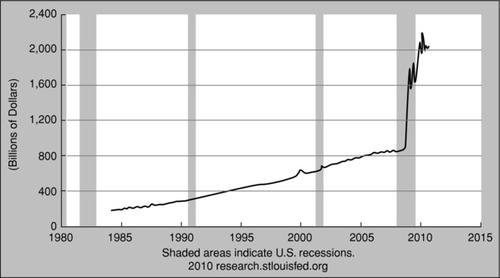
The credit crisis that began in 2007 resulted in a sudden and massive disappearance of liquidity across the entire universe of financial institutions. This was largely, but not entirely, due to a sudden collapse in the values of many mortgage-backed securities and other “hard to price” financial assets, and the disappearance of bidders, making valuations exceedingly difficult. The crisis, as crises often do, fed on itself, and the situation grew progressively worse at an alarming rate. The Fed responded to the crisis by using its tools, primarily open market operations, to dramatically expand the monetary base. It did this by buying up literally hundreds of billions of dollars of securities—eventually reaching into the trillions. These included both agency MBS and Treasuries. Indeed, over just three years, the Fed's balance sheet ballooned by some $2 trillion. The explosive growth of the monetary base can be seen in Exhibit 13.1.
Beginning in December 2007, the Federal Reserve sequentially introduced a number of new, temporary, monetary policy tools in an effort to restore liquidity to financial institutions. These tools represented “innovation on the fly.” Three of these tools were the Term Auction Facility (TAF), the Term Securities Lending Facility (TSLF), and the Primary Dealer Credit Facility (PDCF). All of these have now expired, but they are worth a brief mention as they, or programs like them, could be brought back in short order.
The TAF was a credit facility that allowed banks to borrow from the Fed for periods of 28 days using a wide variety of collateral. When the Fed lends in this way, it credits the borrowing institution's reserves (a liability for the Fed) while simultaneously adding the collateral to the Fed's assets. While Fed lending against collateral increases both the Fed's assets and liabilities by equal amounts, it also has the effect of increasing the monetary base by increasing bank reserves. If the Fed does not wish to see the monetary base expand, it can counteract the effect through open market operations.
The TSLF program allowed prime dealers to borrow Treasuries from the Fed in exchange for less liquid collateral, such as mortgage-backed securities. It was a sort of bond-for-bond swap of securities that did not increase or decrease reserves but did help to restore liquidity to certain key financial institutions. These bond swaps were, like TAF, for periods of up to 28 days.
The PDCF was a cash-for-bonds program that provided funding for prime dealers for up to 120 days. The program accepted a wide variety of collateral. Like TAF, these loans against collateral increased both the Fed's assets and liabilities. They also added to bank reserves. Again, if the Fed did not wish these loans to increase the monetary base, it could take offsetting actions through open market operations.
A fourth tool amounted to the extension of open market operations to include the purchase of agency MBS (i.e., issuances of Ginnie Mae, Fannie Mae, and Freddie Mac) in much the same manner as the purchase of Treasuries. This program is separate and distinct from the U.S. Treasury's Troubled Asset Relief Program or TARP. TARP is not, technically, a Federal Reserve policy tool. It is a program of the U.S. Treasury department that allows the Treasury, in consultation with the Fed and with timely notice to various congressional committees, to purchase troubled assets—primarily residential and commercial mortgage-backed securities. The goals behind the TARP program were to allow banks to get these troubled assets off their balance sheets, restore liquidity to this segment of the financial markets, and to encourage banks to begin lending again. Clearly, these are goals the Fed shared.
As the mortgage-backed securities that the Fed holds have gradually paid down (i.e., principal returned), the Fed has stated that it may reinvest the proceeds into Treasuries. This concerns many economists as it represents a monetization of the national debt with serious long-term inflationary potential.
So What Is It: Inflation or Deflation?
Despite the fact that there is near universal agreement among economists with respect to all three of the key monetary equations noted earlier in this paper and repeated below, economists still disagree as to whether the developed world is headed down an inflationary or a deflationary path. Oddly both are distinct possibilities.
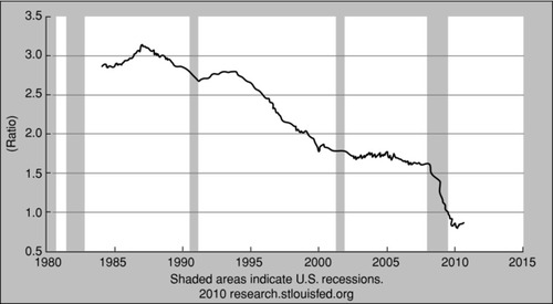
To see how this can be so, consider the equation for the money multiplier. The money multiplier declines if banks choose not to lend so that their excess reserves (e in the money multiplier equation) rise. It is no secret that banks have become skittish and have dramatically reduced their willingness to lend and have raised their lending standards. The latter is not necessarily a bad thing; it is certainly preferable to making uncollectible loans, but it does reduce the money multiplier. Indeed, as of this writing, U.S. bank excess reserves have reached an unprecedented level of $1 trillion. All other things being equal, a reduction in the money multiplier will reduce the money supply for any given monetary base. As a consequence, even though the U.S. monetary base has grown at an explosive rate (ranging from 20 percent to about 100 percent per annum) over the past few years the actual money supply, as measured by M1, has grown at a much slower rate (ranging from 0 percent to about 17 percent per annum) over the same period. Will this continue? Not indefinitely, of course, but for how long is open to debate. The dramatic decline in the money multiplier over the past few years is evident from Exhibit 13.2.
While you might argue that the Fed can compensate by increasing the monetary base further, that is actually very difficult to do. Increasing the monetary base in part requires that banks be incentivized to expand their reserves. The Fed would normally accomplish this by lowering interest rates (i.e., its target Fed funds rate and/or the discount rate). But with the target Fed funds rate nearly zero, there is little more that the Fed can do without literally giving away money. Thus, banks’ reluctance to lend can, in the short run, bring about a shrinkage, or at least very slow growth, in the money supply even as the monetary base continues to expand. This shrinkage in money supply can bring on a bout of deflation. In the longer term, however, when banks do finally begin to lend aggressively and the excess reserve ratio trends back toward zero, the money multiplier can be expected to rise dramatically. This in turn could bring about a rapid expansion of the money supply and, eventually, a serious bout of inflation.
Now consider the equation of exchange. In our earlier discussion of the effect of an expansion of the money supply on the price level and/or real GDP, we assumed that the velocity of money is constant. But, in fact, it is not. It is very much influenced by how people feel about their personal wealth status, their employment prospects, and their perceptions of future prices. Specifically, when people feel “poorer” they tend to dispense with some of their discretionary spending, increasing their savings rate, and thereby reducing velocity. When unemployment rates rise or are high, people also slow down their spending due to job insecurity concerns. This, too, contributes to a decrease in the velocity of money. Finally, if people believe that prices will decline, they tend to postpone consumption in order to get a better price later. This also decreases the velocity of money. Of course, the opposite is also true—as people feel wealthier, as unemployment rates fall or remain low, and as inflationary expectations rise, the velocity of money increases.
Given that at least two of these velocity drivers have been driving velocity lower; that is, people feel poorer due to declines in real estate values and stock portfolios and employment prospects are bleak, we would expect the velocity of money to have declined even if people have no opinion about future prices. Their view on future prices could either mitigate or reinforce these velocity effects. Indeed, in recent years, the velocity of money has been trending downward: between 2008 and early 2010, the velocity of M1 declined by more than 20 percent. The trend in velocity has recently turned modestly upward, but it is as yet unclear if this is the start of a new trend or if the downward trend will resume.
So now consider the implications of a flat money supply despite a rising monetary base and a simultaneously declining velocity of money. If output, that is, real GDP, grows, price levels must fall and a bout of deflation is most likely. If output declines, it could absorb some of the pressure on prices, but it would also likely result in a further exacerbation of the unemployment rate, and this, in turn, could further slow the velocity of money. In other words, a downward spiral in the price level becomes a distinct possibility with further increases in unemployment. This is the classic liquidity trap.
On the other hand, sooner or later it can be expected that the economy will return to its long-term growth path—though this is far from certain as foolish government “fixes” can actually prolong the problems. When this happens the money multiplier will rise dramatically thereby increasing the money supply from a now very high base, and consumers would likely return to their old spending habits with a concurrent increase in velocity. Unless the Fed is able to shrink the bloated monetary base, potent inflation would then be in the offing.
The conclusion is—it could go either way. But deflation seems a more likely shorter-term scenario while inflation seems a more likely longer-term scenario.
EXPRESSING A VIEW: INVESTING WITH PRICE INSTABILITY
How can one position oneself to benefit from his or her monetary outlook? Consider first the prospect of inflation. Here there are several old standbys. During inflationary periods, durable commodities tend to hold their value quite well. This is especially true for precious metals like platinum, gold, and silver. In September 2010 gold hit an all-time historic high, suggesting clearly that not all the world foresees deflation. Even if an investor expects a period of deflation to be followed by serious prolonged inflation, gold and other hard commodities would be a viable hedge. Adding a little leverage changes the outcome, if the view proves right, from a purchasing-power hedge to a very rewarding investment. A number of well-known hedge fund managers, including George Soros, Leon Cooperman, John Paulson, and Erich Mindich, have all purchased gold bullion and/or gold ETFs for their funds, such as SPDR Gold Shares (GLD).
A different approach would be to buy financially-engineered securities specifically designed as a hedge against inflation. Certain types of structured securities serve this purpose well. Examples would be inflation-indexed notes and bonds. The Treasury version, called Treasury Inflation Protected Securities (TIPS), do have some hidden tax traps caused by phantom income, but they offer the credit safety of Treasuries. Corporate inflation-linked bonds and notes do not, generally, suffer from the phantom income problem, and they offer higher yields because they carry greater credit risk. In both cases, however, these products can be shown to be a combination of a traditional bond and a macroeconomic derivative (discussed later). For aggressive investors, new ETF products couple the inflation-indexed products with leverage, allowing them to truly profit from inflation, not just protect their wealth from a loss of purchasing power.
In a serious inflationary environment, interest rates eventually rise dramatically. This causes bonds with fixed coupon rates to lose value. Thus, an inflationary view can be expressed by shorting bonds or, equivalently, by buying a bond ETF specifically structured to be bearish on fixed coupon bonds. This is accomplished with a little financial engineering.
For those with a deflationary outlook, all of the aforesaid strategies can be reversed. However, given how low bond yields have fallen, it is doubtful that there is much upside in an investment-grade long bond position unless considerable leverage is applied. But, that is, of course, what hedge funds tend to do. Paul Broyhill, who runs Affinity, took that approach. Some large hedge funds have, in recent months, been buying up high yield (i.e., junk) bonds, reasoning that those bond yields have further to fall if the deflationary scenario comes to pass—as they expect. One example of this mindset is David Tepper, who runs Appaloosa Management.
MACROECONOMIC DERIVATIVES
Perhaps a purer approach to playing the inflation/deflation views, as well as other novel economic scenarios, is to structure appropriate macroeconomic derivatives (sometimes called economic derivatives).4 These sorts of products were proposed by a number of financial theorists/practitioners over the years including Marshall et al. (1992) and Shiller (1993). But it wasn't until a decade later that derivatives dealers and derivatives exchanges began making markets in these novel products.5
A macroeconomic derivative is a derivative instrument (i.e., swap, option, forward, or futures) contract that is linked to a macroeconomic index of some sort. One could argue that certain commodities have such a broad impact on economic activity that they could be considered macroeconomic indexes. Some would feel this way about the price of crude oil and, therefore, oil futures and oil swaps would be macroeconomic derivatives. Here, however, we take the definition a bit more literally to include only those derivatives written on macroeconomic indexes. These indexes would include such things as inflation rates, unemployment rates, non-farm payrolls, GDP growth rates, real estate indexes, and so on.
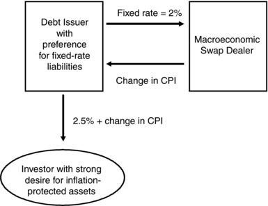
While macroeconomic derivatives have not yet attracted a great deal of attention and the market is still in its infancy, they nevertheless have interesting theoretical and practical applications. Indeed, some of the more popular financially-engineered products, such as inflation indexed bonds, can be shown to be a combination of a straight bond and a macroeconomic swap—specifically, an inflation swap. Suppose, for example, that a bond issuer prefers to issue a straight bond (i.e., fixed coupon, fixed maturity, no embedded optionality) but knows that there is a strong demand on the part of investors for inflation-protected debt products. Specifically, consider the issuer in Exhibit 13.3. It enters into an inflation swap to convert its fixed rate to an inflation-linked rate. The inflation-indexed bond costs the issuer a fixed rate of 4.5 percent per annum: 2 percent is paid to the swap dealer in exchange for the inflation rate, which, in turn, is given to the investor along with an additional fixed rate component of 2.5 percent.
Exhibit 13.3 Engineering an Inflation-Linked Bond
These sorts of structures run the risk of negative inflation (i.e., deflation) so that the change in the CPI component could be negative. Indeed, if the deflation rate were to exceed 2.5 percent, the coupon to the investor would be negative. This can be avoided by embedding an option in the swap and in the note so that the CPI would have a floor of –2.5 percent. (This would likely entail some reduction in the fixed rate component of the note to pay for the option.) This is the same process by which various types of principal-protected equity-linked notes and commodity-linked notes are created.
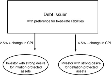
Alternatively, in an environment such as the present in which views are strongly split between inflation and deflation, we could have an issuer issue two bonds: one indexed to play the inflation view and one reverse indexed to play the deflation view. This is depicted in Exhibit 13.4. From the investor's perspective, one has an inflation-biased product and the other a deflation-biased product. But from the issuer's perspective, the aggregate issuance is fixed rate.
Exhibit 13.4 Issuer with Offsetting Bonds
While not shown here, the principal can be protected on each of these notes, using an appropriately structured option, and leverage can be added if the investors so desire. For example, the note could pay a fixed rate plus/minus some multiple of the change in the CPI.
Cyclically Sensitive Municipalities (and Corporations)
At the end of August 2010, the city of Harrisburg, announced that it expected to default on its debt by missing a $3.9 million interest payment. Harrisburg is the capital of the Commonwealth of Pennsylvania. Actual default was averted, at least temporarily, when the Commonwealth of Pennsylvania announced a week or so later that it would accelerate some grants and other payments to the city to allow Harrisburg to meet its upcoming debt service. The bonds are insured by a municipal bond insurance company, so investors were not at significant risk, but a default would drive up Harrisburg’s, and other municipalities’, future funding costs. At the time of this writing, the cities of Detroit, Michigan, and San Diego, California are in similar straits.
The problem for these three municipalities, and almost all others as well, is that any economic slowdown will cause a decline in their tax revenues while increased community needs will make greater demands on the expenditure side. Almost all municipalities are cyclically sensitive. But the degree of cyclicality varies considerably from locale to locale. A city that is home to many cyclically sensitive businesses will itself be particularly cyclically sensitive. A city that is dominated by colleges and universities will be less impacted, at least for a time, by economic stress.
Given this cyclical sensitivity, one might be inclined to think the solution is simple: Municipalities should build reserves during expansionary periods in order to have a rainy day fund to draw on during periods of contraction. But history proves that few municipalities can do this. Politicians are always under pressure to show the voter that they are conscious of the voters’ concerns—especially with respect to taxes. Surpluses are hard to justify as they lead to pressure to either (1) increase spending, (2) cut taxes, or (3) some combination of the two.
Macroeconomic derivatives could easily represent a powerful, albeit partial, solution to this problem. Using historic data, a city like Harrisburg should be able to determine how changes in national or regional GDP growth impact its cash flows. Alternatively, it might do the analysis using the national or a regional growth rate in non-farm payrolls. The city could then enter into a GDP or non-farm payroll swap. We will use the GDP swap to illustrate the process.
Let's suppose that a city's risk management committee (RMC) knows from experience that the municipality's budget is balanced when the real economy grows at 2.7 percent—which is the official estimate of the long-term real GDP growth rate. The RMC (or an outside expert hired for that purpose) has further determined that a one percent change in GDP translates into $20 million of net cash flow for the city. That is, for every one percent increase in GDP the city will have an annual extra $20 million of net cash flow. (Net cash flow is the difference between revenues received and the sum of budgeted and unbudgeted expenditures.) Conversely, for every one percent decrease in GDP, the city will suffer an annual $20 million decrease in net cash flow. When the city is in a cash surplus state, it experiences pressure from special interest groups to spend more and from taxpayers to cut rates. When the city is in a cash deficit state, pressure mounts to raise taxes (always politically unpopular), spend more on social safety net programs, and borrow in the capital markets. The goal is to keep the city's budget balanced in all economic climates.
So the city enters into a 10-year GDP-swap with a macroeconomic swap dealer that uses the same estimate of 2.7 percent long-term real economic growth as measured by GDP. This growth estimate is used to price the swap. Suppose that they structure the swap such that the city pays the swap dealer the actual annual growth rate in GDP on notionals of $2 billion and the swap dealer pays the city an annual fixed rate of 2.7 percent on the same $2 billion of notionals. Note two things: First, the notional principal is not real money, and no one gives this to the other—it only exists for purposes of calculating the later periodic payments. Second, in practice, there would be a spread, measured in basis points, on the GDP leg to compensate the dealer for its role in the swap, but we will ignore that in this example. The structure of the swap, together with the municipality's cash flows from taxes and expenditures, is depicted in Exhibit 13.5.
Exhibit 13.5 A Macroeconomic Hedge

The beauty of the swap solution is that the city is now insulated (i.e., hedged) against a large portion of its macroeconomic (a form of systemic) risk stemming from the cyclicality of the city's cash flows. Importantly, the city would not want the swap to have a very long tenor because a city's internal dynamics change over time and the degree of cyclicality may be impacted by that change. To see that the swap works, suppose that the economy's growth rate increases to 3.7 percent. Then, under the terms of the swap, the municipality would pay the dealer $74 million (i.e., 3.7 percent × $2 billion), and the swap dealer would pay the city $54 million (i.e., 2.7 percent × $2 billion). In a swap, only the net is exchanged with the higher paying party paying the lower paying party the difference. So, in this case, the city pays the swap dealer $20 million—which is precisely the size of its surplus for the year. On the other hand, suppose that the following year the economy sinks into a recession and GDP growth becomes negative, say –1.3 percent. Then, the swap dealer will pay the city $26 million on the GDP leg. (This is because the payment on the GDP leg is negative, so it goes in the opposite direction.) And the swap dealer also pays the city $54 million on the fixed leg. Thus, the city receives an infusion of $80 million from the swap dealer thereby offsetting its cash flow shortfall caused by the decline in GDP (i.e., the recession).
One of the beautiful things about this solution to a municipality's cyclical macroeconomic risk is that it would likely remove much of the political pressure to increase spending in good economic times and decrease pressure to raise taxes and cut services during poor economic times. Thus, it fosters an environment of stability, which facilitates long-term municipal planning.
Macroeconomic swaps (and other macroeconomic derivatives) are not as easily constructed as we might have led you to believe. In the swap market, dealers act as intermediaries between end users. To function well in this capacity, there needs to be a two-way market. Of course, there are far more corporations and municipalities that are cyclical than counter-cyclical, so one might argue that the market cannot work. But, there are ways around this problem as has been demonstrated by the Case-Shiller real estate indexes. These indexes became the basis of futures contracts and swap dealers can hedge in the futures. It only requires that there be sufficient speculative interest on the other side of the futures contracts. There are, of course, other problems with swaps of this nature, such as how to handle revisions in the GDP number, which can happen several calendar quarters out. But those sorts of issues are resolvable by employing appropriate lags.
Another solution, which really involves an embedded swap, very much the same way that the inflation-indexed bonds involve an embedded swap, is to structure municipal debt offerings with a floating coupon such that it is tied inversely to the growth rate of GDP. For example suppose that, under current market conditions, our aforementioned city could issue a 10-year note paying a fixed rate of 5 percent. Instead, suppose they issue a note paying 2.3 percent plus the growth rate of real GDP. If the long-term growth rate of GDP turns out to be 2.7 percent, then on average, the city has paid an annual coupon of 5 percent over the 10 years. But in years when GDP is above its long-term estimated growth rate, they pay more and in years when GDP is below its long-term estimated growth rate, they pay less. This sort of debt financing would have negated the need for the city of Harrisburg to announce that it was going to miss an interest payment. Indeed, this sort of debt financing would likely lead to a long-run increase in the debt rating of the city. Rating agencies would see the city's finances as more economically stable. This, in turn could lead to an even lower fixed rate component. For example, the coupon might be 2.1 percent plus the GDP growth rate.
In concluding this chapter, we hope that we have demonstrated that there is lots more room for financial innovation and financial engineering. If done right, it can help address systemic problems that have plagued municipalities and corporations alike since the birth of the modern state.
NOTES
1.The importance of a strong figure at the helm of a central bank is well documented in Ahamed (2009).
2.The monetary base is also known as base money, high-powered money, and reserve money.
3.Of course, it is possible for an increase in the money supply, assuming velocity is constant, to show up as a decline in P or Q but a more than offsetting increase in Q or P.
4.We prefer the term macroeconomic derivative to economic derivative. In a sense, all derivatives serve an economic purpose and could therefore be loosely called economic derivatives, but not all derivatives can be macroeconomic in nature. For example, a futures contract on a commodity price is “economic” in nature, as the prices of all commodities are determined by the laws of supply and demand. This would generally be “microeconomic” but still economic. The term macroeconomic derivatives makes clear that we are talking about a derivative on a macroeconomic variable. Admittedly, it is sometimes difficult to draw the line between what is microeconomic and what is macroeconomic.
5.In the early 2000s, Deutsche Bank and Goldman Sachs collaborated in creating a market in over-the-counter macroeconomic derivatives. Similarly, several futures exchanges have introduced macroeconomic index based futures contracts.
REFERENCES
Ahamed, Liaquat. 2009. The Lords of Finance. London: Penguin Press.
Bansal, Vipul K., J. F. Marshall, and R. P. Yuyuenyongwatana. 1995. “Macroeconomic Derivatives: More Viable than First Thought!” Global Finance Journal 6:2, 101–110.
Blaise Gadanecz, R. Moessner, and C. Upper. 2007. “Economic Derivatives.” Bank for International Settlements, BIS Quarterly Review, March.
Gurkaynak, Refet, and J. Wolfers. 2006. “Macroeconomic Derivatives: An Initial Analysis of Market-Based Macro Forecasts, Uncertainty, and Risk.” NBER Working Paper No. 11929.
Marshall, John, F. V. Bansal, A. F. Herbst, and A. L. Tucker. 1992. “Hedging Business Cycle Risk with Macro Swaps and Options.” Continental Bank Journal of Applied Corporate Finance 4:4, 103–108.
Shiller, Robert. J., 1993. Macro Markets: Creating Institutions for Managing Society's Largest Financial Risks. New York: Oxford University Press.