
Appendix A
IT Tools for Financial Asset Management and Engineering
INTRODUCTION
The study of finance concerns itself with both theoretical and practical issues. The relationship between the volatilities and correlations of individual securities, and the volatility of a portfolio consisting of those securities, is an example of a theoretical issue, whereas the speed with which a stop loss order can be executed once it has been triggered is an example of a practical issue. Theoretical issues and practical issues are, of course, not necessarily independent of one another, but they are typically addressed by different groups of people. The solution to theoretical problems typically leads to efforts to implement the theory and that, in itself, can pose a number of computational problems. These computational problems can often be addressed with the aid of appropriate information technology (IT) tools. In this appendix, we will consider the role these tools can play in addressing computational problems. In the process we will touch on modeling tools, mathematical/statistical tools, and data tools. Numerous books have been written on each of these types of tools and this short appendix cannot possibly do these tools justice. But we hope that the new student of financial engineering will get a sense of what is available when he or she encounters problems where these tools may have a use.
In general, we can distinguish among four classes of problems:
1. Problems that are hard to solve because we do not have enough time or computing power to solve them.
2. Problems that are hard to solve because we do not understand how to solve them.
3. Problems whose parameters are constantly changing, resulting in a need for constant updating.
4. Problems wherein having accurate and well-defined input data is key.
Importantly, these classes of problems are by no means mutually exclusive; there is much overlap.
We will consider an example of each type of problem and illustrate approaches and tools that have proven useful in addressing them. It will come as no surprise to the reader that the principal tool will be the computer. But, more broadly, it is the whole computational/information-system infrastructure that has developed over the past 20 years that is key. Specifically, this includes the personal computer, the local area network, the Internet, and the software used to manage these things.
Let us begin by considering a problem of the first type (i.e., a problem that we know how to solve, but we do not have the necessary time and/or computational resources). Imagine, for the sake of argument, that we have a large pool of subprime mortgages. Let us suppose that each of these mortgages has the same probability of going into default and subsequent foreclosure. Further, let us suppose, for simplicity, that the mortgages default independently of each other (i.e., that the cross default correlation is 0). Thus, given independence, the joint probability that, for example, any two of these mortgages, xi and xj, defaults is simply given as follows:
![]()
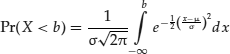
Where Pr(xi,xj) denotes the joint probability of default and Pr(xi) and Pr(xj) denote the individual probabilities of default for xi and xj respectively. Because the probability of default is the same for each mortgage, let's denote this probability simply by p. So far, so good. Now let's add some meat to the problem. Suppose we have a very large pool consisting of 100,000 equal size mortgages and the probability of any one mortgage defaulting over the coming year is 0.05 (i.e., 5 percent). Now consider a mortgage-linked product whose payoff is based on the behavior of this pool. More specifically, suppose that it is a barrier option that will pay off if and only if the number of defaults over the next year, denoted by X, falls within a specified range whose lower bound is a and whose upper bound is b. That is, we are interested in the probability that X, the total number of defaults, will lie between a and b. That is, we seek to find Pr(a < X < b).
In this case, the problem is well understood by statisticians as having a binomial distribution, and the answer, therefore, is given as follows:
![]()
Finally, let's suppose that a = 5,100 and b = 10,100. Now, the issue is this: If the number of mortgages in the pool was small, anyone with a scientific calculator could perform this operation. However, in our example, n = 100,000 and i may range from 5,100 to 10,100. Among the many computations that need to be made is this one (which is just part of the first term in the summation):
![]()
Plugging this into a TI-83 calculator would result in the following: ERR: OVERFLOW. And this is only the first of 5,000 similar computations needed to find out the probability of having between 5,100 and 10,100 defaults.
The issue is not one of theory, but rather one of computing power. The TI-83 does not have the capability, but the more powerful TI-89 does. Nevertheless, there are still 4,999 similar computations to do. Even if each computation could be done in just 30 seconds, it would still take more than 40 hours to achieve a viable solution. A derivatives trader requires an answer in a fraction of a second! Thus, an understanding of theory alone is not helpful to the trader.
This particular problem has an easy solution, and we can use it to illustrate, first, how theory can inform on issues of computability and, second, how certain features of common software can be used to solve the problem even faster.
Statistical theory tells us that a binomially distributed random variable can be approximated by a normally distributed one, where μ = np and σ = [np(1 – p)]1/2. Thus, the computation above can be well approximated by:
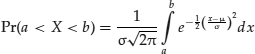
Now, at first blush, this seems worse than before. However, the ubiquitous MS-Excel® is actually capable of solving this problem in one step.1
BASIC MS-EXCEL® TOOLS
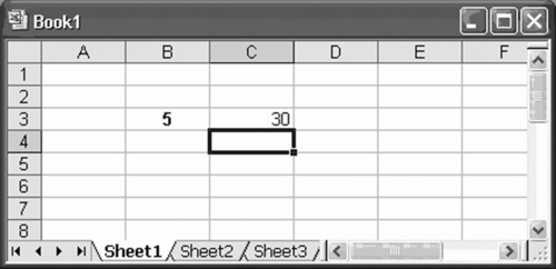
MS-Excel has a huge amount of computational power built into it and we shall examine several of its features. But, first, let us finish the problem. In MS-Excel, one would enter the expression:
![]()
That is, provided we can assume normality, MS-Excel comes preprogrammed to solve complex integration problems for us. In this case, the solution is 7.34 percent. Thus, we conclude that there is a 7.34 percent probability that the option will pay off.
Other preprogrammed features that are particularly useful in financial modeling include arithmetic means, geometric means, standard deviations, variances, maximal/minimal element (of a set), binomial distributions, matrix computations, and correlations, as well as a complete Visual Basic programming environment. These represent only a tiny fraction of the tools available, and we will use some of them in the following examples. For the reader who has little to no experience with MS-Excel modeling, it is useful to know that the software provides an extensive “Help” reference with detailed instructions. If one does not know the name of a particular MS-Excel function, or is unsure of which function is appropriate, one can select “Function” from the “Insert” menu (alternatively, one can click the fx icon toward the top of the worksheet area). This allows you to navigate to the appropriate function, and will tell you the function's arguments.
Suppose we wish to compute the average rate of return over a period of years given a list of the n individual yearly rates, ri. In this case, the average rate is given by:
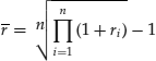
One can solve this in MS-Excel, by utilizing the function =GEOMEAN(). In a new column or row, simply add 1 to each annual rate. Then use the GEOMEAN function on this new series, and subtract 1 from the result to obtain the geometric mean rate.
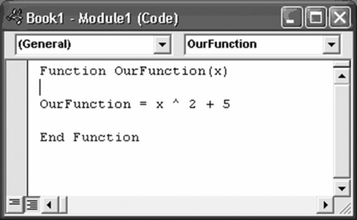
If there is a specific function that you expect to employ frequently and MS-Excel does not include it as one of its built-in functions, you can simply create it. This is called a “user-defined function,” and it is created using the Visual Basic Editor. We will demonstrate this with a simple example. Suppose we wish to define a function, which we will name “OurFunction,” that squares a number and then adds 5 to it. In other words:
![]()
We simply go to the “Tools” menu, navigate to “Macros,” and open the “Visual Basic Editor.” A screen opens where we insert a module as shown in Exhibit A.1.
Exhibit A.1 Creating a User-Defined Function
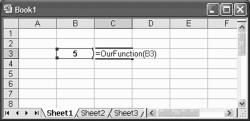
Now, we close and return to MS-Excel. We have just constructed a simple function that we can use by going to any cell in our spreadsheet and entering it as shown in Exhibit A.2.
Exhibit A.2 Employing a User-Defined Function
The result is shown in Exhibit A.3.
Exhibit A.3 Output Generated by the User-Defined Function
MATHEMATICA®, GAUSS™, MAPLE®, AND MATLAB®2
Computers have long been able to assist researchers, analysts, and engineers with numerical computation, such as the approximation of a definite integral, that were previously performed by hand. But symbolic computation, also known as algebraic computation, was not, until recently, similarly readily available. Thus, systems of equations had to be solved by hand, difficult integrals had to be looked up on tables, similarity methods had to be employed to obtain solutions to partial differential equations, and so forth. While we are not yet free of the need to think about these things, Mathematica, Gauss, Maple, MatLab, and other symbolic computation engines are now available and can be used to great effect. We will use Mathematica for purposes of illustration in this section.
First, let us recall the straightforward but complex integration from before—that is, computing the cumulative distribution function (cdf) of the normal distribution:
In Mathematica, one enters the integral symbolically as shown:
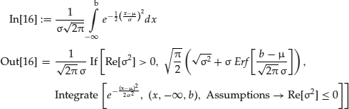
Mathematica does not know what we are doing and therefore warns us that the variance must be positive. However, it correctly computes the cdf, after canceling a few terms, as:
![]()
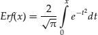
where Erf is the Gaussian error function:
If one wishes to find the first few terms of the Taylor Series approximation for this function around the point x = a, in Mathematica one simply enters the problem in symbols as shown:
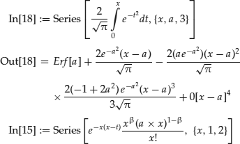
Here, Series[f, {x, x0, n}] generates a power series expansion for f about the point x = x0 to order (x − x0)n.
BLOOMBERG®3, INFORMATION, AND THE API
So far we have seen that with the use of software we can solve problems of the first two types. That is, we can solve (1) problems that are difficult to solve due to time constraints or insufficient computing power, and (2) problems that are hard to solve because we do not understand how to solve them. We now turn to the third type of problem: those whose parameters need constant updating.
In finance, we are often confronted with data sets that are constantly changing. Quotes, for example, on liquid instruments can change by the millisecond. Even if one has constructed a model wherein the theory is sound and where issues of computability have been resolved, a lack of current data may still block our path to a solution.
Consider California in 1849. Gold was discovered at Sutter's Mill in 1848 and by 1849 the gold rush was on. Some prospectors, of course, became rich, but the majority did not. Most, in fact, did not find any gold. There is one thing, however, that almost every prospector did do: He bought a shovel. Thus, selling shovels was a less exciting but more reliable business to be in than prospecting. This is the principle that Michael Bloomberg understood in the 1970s. He realized that although most investors would not get rich in the (then) new computer era, almost all would demand up-to-date information. Thus, in the spirit of Reuters, Bloomberg founded his company to sell financial information terminals to Wall Street. To make a long story short, his net worth is now over $10 billion.
The Bloomberg terminal is the financial engineers’ shovel. With this terminal he or she gains not only real-time trading data, but also analysis, news, and much more. However, it provides such a vast amount of information that one can be lost before one even begins. Being able to look up all this data is wonderful, but the real power of the Bloomberg system is only fully realized when the information-retrieval services it offers are married to modeling software that takes the data as input. In this section, we describe some of these features.
When a Bloomberg account is opened, it is important that a feature called API be activated. API stands for Application Programming Interface. It is the bridge that allows a Bloomberg terminal to “talk” to MS-Excel.
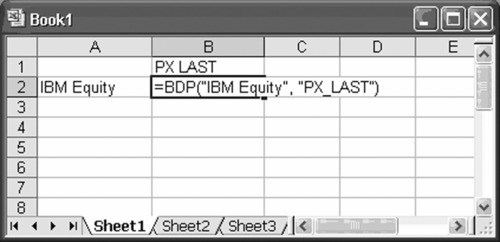
Data requests may be specified either by selecting appropriate options from the Bloomberg menus or by entering direct codes. For example, a direct code might look like Exhibit A.4.
Exhibit A.4 Direct Code to Retrieve the Last Trade Price for IBM
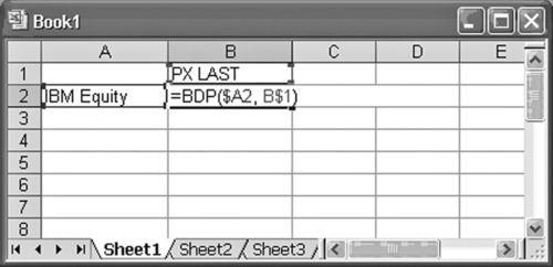
Alternatively, one could incorporate cell references in the code to achieve the same result. This is illustrated in Exhibit A.5 for the same example employed in Exhibit A.4.
Exhibit A.5 Direct Code Incorporating Cell References
Through the API, we can easily and quickly populate an entire table with real-time data. Much more complex information is also accessible. For example, the BDS (Bloomberg Data Set) command returns multicell descriptive data to your MS-Excel spreadsheet using the following syntax:
![]()
The “security” entry may be any valid identifier such as a ticker symbol or a ticker/exchange, CUSIP, or ISIN, followed by the relevant sector indicator (e.g., Equity or Corp). The “field” indicates the type of information you want (e.g., last bid, etc.). Last, the optional arguments are for settings that may have particular relevance, but are not needed. Committee on Uniform Security Identification Procedures (CUSIP) numbers are used to identify North American securities. International Securities Identification Numbers (ISINs) are similar in function.
Almost any sort of information may be retrieved in this way. Thus, with a Bloomberg terminal, the only limits on data inputs are the limits of one's own imagination. Since the API software updates continuously, real-time model creation is straightforward.
MORE COMPLEX MS-EXCEL COMPUTATIONS
We have already discussed a number of MS-Excel's useful features. The following list expands on this a bit.
Use Tools|Data Analysis|Descriptive Statistics to compute the descriptive data.
Use Tools|Data Analysis|Correlation Analysis to compute the correlation matrix of an n-return series.
Use Tools|Data Analysis|Histogram to compute either an empirical distribution of data or the cumulative distribution of data.
Use Tools|Data Analysis|Linear Regression to perform regression.
MS-Excel can also do matrix computations. The following matrix functions are available:
Use MMULT to compute matrix products.
Important Note: In matrix operations, one must highlight the matrix and type Ctrl-Shift-Enter to validate.
Use TRANSPOSE to compute the transpose of a matrix.
Use MINVERSE to compute the inverse of a matrix.
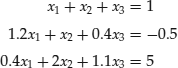
As a first example of the manipulation of matrices, consider the problem of solving the following system of linear equations:
Note that if the matrix of the coefficients (A) is square and nonsingular, the system AX = Y always has a unique solution. The solution to the system is found by premultiplying both sides of equation AX = Y by the inverse of A: AX = Y ⇒ A-1 AX = A-1 Y ⇒ X = A-1 Y.
A is the coefficient matrix, X is a column vector containing the unknowns for which we seek a solution (x’s), and Y is a column vector of constants (numbers at the right-hand side of the equations).
Thus, in MS-Excel, we have Exhibit A.6 and Exhibit A.7.
Exhibit A.6 Original Matrix and Inverse Matrix with Solutions Showing Inverse Matrix Function
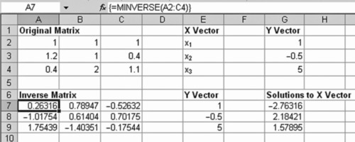
Exhibit A.7 Original Matrix and Inverse Matrix with Solutions Showing Matrix Mutliplication
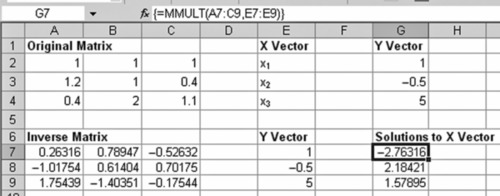
The solution is: x1 = - 2.76316,x2 = 2.18421,x3 = 1.57895.
Now, for a more complex application, we return to our example of a basket of risky mortgages. We are interested in building a model of credit default for the entire structure. Several steps along the way are of particular interest to us as they exemplify methods introduced earlier. Specifically, we use Robert Merton's definition of default, wherein default occurs when the size of the debt exceeds the value of the asset. In Merton's (1974) model, asset valuation may be expressed as follows:
![]()
Where Vt denotes the value of the asset, and V0 denotes the value of the debt (i.e., debt principal), and z is a Weiner process, such that z ∼ N(μ,σ).
It can be shown that the probability of default, given the preceding definition of default, may be expressed as:
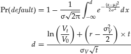
The value and implied risk probability, at any moment, are found using the following MS-Excel expressions (employed in the spreadsheet depicted in Exhibit A.8):
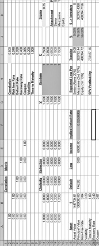
Exhibit A.8 Model of Default
![]()
Note that d is simply the upper limit of the integral shown, i.e., the cumulative normal distribution. For simplicity, we assume a simple mortgage-backed security (MBS) structure with only five reference assets (mortgages) and three tranches: equity, mezzanine, and senior, absorbing the bottom 10 percent, the second 10 percent, and the last 80 percent of the default risk, respectively. We relax our earlier assumption of no cross default correlation.
We assume that a default event has occurred when Vt < V0. In this case, the loss to the special purpose vehicle (SPV) is given by Li = (1 - δi )V_t, where δi is the recovery rate for the ith asset, which is allocated to the lowest tranche first.
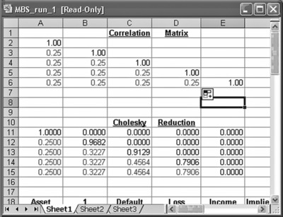
The problem is that we wish to incorporate contagion and/or hedging effects; so, we assume an initial correlation matrix:
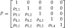
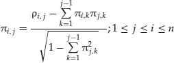
We now compute the Cholesky transformation, Π, which is defined as:
A convenient property of the Cholesky transformation is that given a vector, z = (zi), of n random numbers drawn from a standard Gaussian distribution, then for ρi,j = k, the vector c = P × z is a vector of n random numbers that are correlated with ρi,j = k.
By substituting c for z in the preceding valuation equation, we can generate default events with known correlation. Further, by using Monte Carlo simulation, we can determine an appropriate pricing structure for each of the tranches.
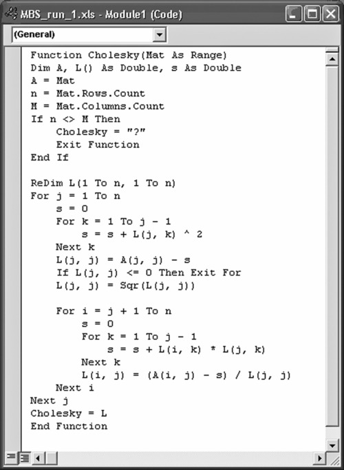
Even with MS-Excel's predefined functions, this matrix would be tedious to compute. Therefore, we use the VB program shown in Exhibit A.9.
Exhibit A.9 VB Code to Automate Cholesky Transformation
The result is shown in Exhibit A.10.
Exhibit A.10 VB Generated Cholesky Reduction
MONTE CARLO SIMULATION
We have seen how modern software can help us solve all four categories of problems that were described in the introduction to this appendix. But there are times when we need to solve a problem when very little is known about the structure of the problem and/or no analytical approach is available. In these situations, Monte Carlo simulation is often an applicable tool. The technique, which is extremely versatile, works by generating random observations on a variable of interest. With a sufficient number of observations, the average tends to converge to the true value of the variable. Importantly, Monte Carlo simulation is also often useful as an alternative approach when we do have an analytical model available. Consider a very simple application. Suppose that we want to know the value of “pi” (denoted π), which is defined as the ratio of the area of a circle to the square of the circle's radius:
![]()
We can easily measure the radius, denoted below by r, but it is far more difficult to directly measure the area of the circle. So let's try to derive the area of the circle via Monte Carlo simulation using nothing more than the built-in functions of MS-Excel. We'll begin by drawing a square such that each side has a length of 1. Next, draw a quarter circle inside the box from the upper left corner to the lower right corner. This is depicted in Exhibit A.11.
Exhibit A.11 A Quarter Circle
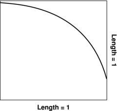
The area of this quarter circle is exactly one-fourth of the area of a full circle. Now imagine that we randomly throw darts at the box in such a fashion that each dart lands in the box with equal probability of hitting any spot in the box. After throwing a sufficiently large number of darts, we can count the number of darts that land within the quarter circle (i.e., below the curve) in Exhibit A.11. Because the length of each side of the box is the same as the radius of the circle, it is clear that the box has an area of 1. The fraction of the total number of darts thrown that land below the curve (i.e., within the quarter circle), then gives us an approximation of the area of the quarter circle. Denote this fraction by g.
But how do we simulate the throwing of darts, such that there is equal likelihood of hitting any spot within the box? The answer is we employ the random number generator in MS-Excel, =RAND(). Each time this is run it will generate a value between 0 and 1 and every possible value is equally likely. If we run =RAND() twice, we can think of the two simulated values as x,y coordinates within the box.
Because we only drew a quarter circle for a circle having a radius of 1, the total area of the full circle having a radius of 1 is 4 × g. Thus, π is approximated by:
![]()
And since, in this case, the radius squared equals 1, the solution becomes:
![]()
In addition to employing the random number generator to generate simulated dart throws, we also employ the counting and logical test features of MS-Excel in the application.
Exhibit A.12 Monte Carlo Simulation of Dart Throws
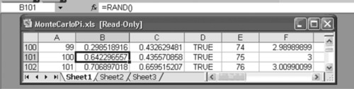
Consider the spreadsheet illustrated in Exhibit A.12. Column A shows the dart count, columns B and C show the x,y coordinates generated using =RAND(). Column D is the logical test: “TRUE” if the dart is within the quarter circle, and “FALSE” if the dart is outside the quarter circle.
Consider dart number 100 (from column A). We can see that the logical test has determined that this dart fell within the quarter circle (as did darts numbered 99 and 101). The logical test function is depicted in Exhibit A.13.
Exhibit A.13 The Use of the Logical Test Function
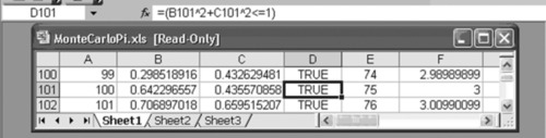
Finally, note that column E provides a running count of the “TRUEs” and column F provides a running estimate of the value of π, by taking the running count of the number of TRUEs,divided by the total darts thrown, and then multiplying this quotient by 4. See Exhibit A.14 for the count function.
Exhibit A.14 Running Count of the “Trues”
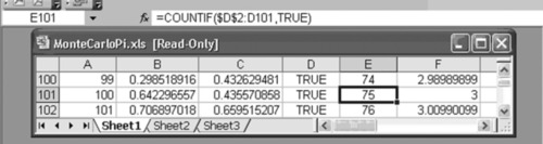
Exhibit A.15 Monte Carlo Simulation Convergence
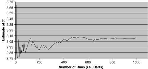
The final exhibit, (Exhibit A.15) shows a graph of the estimate of π plotted as a function of the number of darts simulated. It is easily shown that the larger the number of runs (i.e., simulated darts), the more accurate the estimation. This is typical of the convergence to the true value sought as the number of “runs” increases when employing Monte Carlo simulation.
CONCLUSION
We have seen that modern software allows the financial engineer to attend to multifaceted problems without having to learn complex programming, advanced mathematics, or even much about databases. That does not mean that one should not strive to learn these things, only that, for some purposes, it is not necessary to know them at the same depth that the highly quantitative segment of the financial engineering population does.
Because the length of this appendix does not permit a truly in depth discussion of any one of the techniques illustrated, a useful list of resources has been included below.
READER RESOURCES
Books on Financial Engineering Careers
Derman, Emmanuel. 2004. My Life as a Quant: Reflections on Physics and Finance. Hoboken, NJ: John Wiley & Sons.
Jui, Brett. 2007. Starting Your Career as a Wall Street Quant. Denver, CO: Outskirts Press.
Neftci, Salih N. 2004. Principles of Financial Engineering. New York: Academic Press.
Schachter, Barry, and Richard R. Lindsey, eds. 2007. How I Became a Quant: Insights from 25 of Wall Street's Elite. Hoboken, NJ: John Wiley & Sons.
Financial Modeling Using MS-Excel
Benninga, Simon. 2008. Financial Modeling, 3rd ed. Cambridge, MA: MIT Press.
Mathematica
Stinespring, John Robert. 2002. Mathematica for Microeconomics. New York: Academic Press.
Visual Basic
Bovey, Rob, Dennis Wallentin, Stephen Bullen, and John Green. 2009. Professional Excel Development: The Definitive Guide to Developing Applications Using Microsoft Excel, VBA, and .NET, 2nd ed. Ann Arbor, MI: Addison-Wesley Professional.
Monte Carlo Simulation
Monte Carlo simulation can be implemented using MS-Excel as well as other software packages. One such package is Crystal Ball®, which is published by the Oracle Corp. This software allows the engineer to take any spreadsheet and define his or her input and output variables so that the simulation can be performed. Another popular software product (particularly in the health-care industry) is TreeAge Pro which is published by, and is a trademark of, TreeAge Software, Inc.
Bloomberg
Bloomberg data requires access to a Bloomberg terminal. Once one has access to the terminal, as well as a username and password, the BU command takes you to Bloomberg University, which contains an enormous amount of documentation, as well as access to staff to assist you around the clock.
Other Interesting Sources
NOTES
1. Excel is a registered trademark of Microsoft Corporation.
2. Mathematica is a registed trademark of Wolfram Research, Inc.; Gauss is a trademark of Aptech Systems, Inc.; Maple is a registered trademark of Maplesoft, a division of Waterloo Maple Inc.; and MatLab is a registered trademark of The MathWorks, Inc.
3. Bloomberg is a registered trademark of Bloomberg, LP.
REFERENCES
Chacko, G., A. Sjöman, H. Motohashi, & V. Dessain, 2006. Credit Derivatives: A Primer on Credit Risk, Modeling, and Instruments, Upper Saddle River, New Jersey, Wharton School Publishing.
Merton, Robert C., 1974. “On the Pricing of Corporate Debt: The Risk Structure of Interest Rates,” Journal of Finance 29: 449–70.
ABOUT THE AUTHOR
Lucas Bernard has been working in the financial and risk-management arenas, in their broadest interpretation, for many years. Possessing a varied background ranging from entrepreneurship and small business to academic research and consulting, Dr. Bernard is no stranger to the “real” economy, industry, and engineering. In addition to his PhD in Financial Economics (his doctoral dissertation concerned endogenous models of credit default), from The New School for Social Research (NSSR), he also holds masters degrees in both Mathematics, from The City University of New York (CUNY), and Computer Science, from NYU's Courant Institute of Mathematical Science (CIMS). His business background ranges from urban infrastructure planning and pharmaceutical consulting to franchising and even a “dot-com” start-up. He is also certified as a Financial Asset Manager & Engineer by the Swiss Finance Institute (SFI), a private foundation created by Switzerland's banking and finance community in cooperation with leading Swiss universities. An experienced teacher, Dr. Bernard has taught Statistics, Econometrics, and other financial topics at New York University (NYU), at the Polytechnic Institute of NYU (NYU-Poly), where he is a Research Fellow, and in the MBA program at Long Island University (LIU). His current and full-time affiliation is with The City University of New York, College of Technology (CUNY-CityTech), where he is an Assistant Professor in their Business Department. His personal web page is http://www.lucasbernard.com.