
In this chapter, we will start working with images—images that may come from a variety of sensors carried by satellites, drones, airplanes, and so on. These types of images, the ones collected from remote sensing devices, are images that contain pixels representing a spectral response from a given geographic region.
Besides just adding images to a map, it is important to prepare the images to be presented on the map. You may need to combine, cut, change the resolution, change values, and perform many other transformations in order to produce a visually appealing map or valuable information.
To perform these transformations on the images, we will go through a process of deduction that will result in a versatile and powerful software structure.
The topics covered here are:
- Understanding how the images are represented
- The relation of the images with the real world
- Combining, cropping, and adjusting the values of the images
- Creating shaded relief maps from the elevation data
- How to execute a sequence of processing steps
In order to understand what images are in terms of computer representation and the data they contain, we are going to start with some examples. The first thing to do is to organize your project to follow this chapter's code as follows:
- As before, inside your
geopyproject, make a copy of yourChapter5folder and rename it toChapter6. - Inside
Chapter6, navigate to theexperimentsfolder and create a new file inside it namedimage_experiments.py. Open it for editing.
We will start by inspecting a small sample image that has a structure similar to a large satellite image.
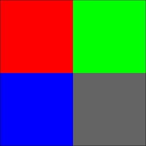
Nothing fancy, you will see four squares of different colors. But if we take a step further and add a grid to it, we can see a little bit more information.
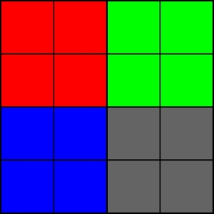
The image was divided into 16 squares of equal size. Each one of these squares is a so-called pixel. A pixel is the smallest portion of information that an image (that is, raster data) contains. While talking about geoprocessing, the image as a whole comprehends a space in the real world and each pixel is a fraction of that space.
When we added the sample image to the map in the beginning of the chapter, we manually defined the extent of this image (that is, its bounding box). This information told Mapnik how the coordinates in the image relates to the real world coordinates.
So far, we have seen that our sample image has 16 pixels with a shape of 4 x 4. But how this image or any other raster data relates to a real world space depends on the information that may or may not be stored in the data itself.
The first information that states the relation is where the image is in the world. Images and raster data normally have their point of origin in the top left corner. If we assign a coordinate to the point of origin, we will be able to place the image on the world.
Secondly, we need information on the area that this image covers. And there are three ways this information can appear:
- The size of the pixels of the image
- The size of the image
- The coordinates of the bounding box of the image
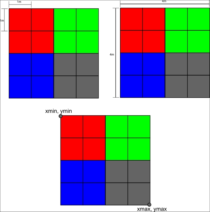
This information is related by the following equations:
x_pixel_size = width / columns
y_pixel_size = height / lines
width = xmax – xmin
height = ymax – ymin
For a better understanding, we will open the sample image with OpenCV and inspect its contents as follows:
- In your
image_expriments.pyfile, type the following code:def open_raster_file(image): """Opens a raster file. :param image: Path of the raster file or np array. """ image = cv2.imread(image) return image if __name__ == '__main__': image = open_raster_file('../../data/sample_image.tiff') print(image) print(type(image)) print(image.shape) - Run the code. Since it's the first time you have run this file, press Alt + Shift + F10 and choose
image_experimentsfrom the list. You should see the following output:[[[ 0 0 255] [ 0 0 255] [ 0 255 0] [ 0 255 0]] [[ 0 0 255] [ 0 0 255] [ 0 255 0] [ 0 255 0]] [[255 0 0] [255 0 0] [100 100 100] [100 100 100]] [[255 0 0] [255 0 0] [100 100 100] [100 100 100]]] <type 'numpy.ndarray'> (4, 4, 3) Process finished with exit code 0
The expression print(type(image)) prints the type of the object that is stored in the image variable. As you can see, it's a NumPy array with a shape of 4 x 4 x 3. OpenCV opens the image and put its data inside an array, although for now, it is a little bit hard to visualize how the data is organized. The array contains the color information for each pixel on the image.
For better visualization, I'm going to reorganize the print output for you:
[[[  0   0 255] [  0   0 255] [  0 255   0] [  0 255   0]]
 [[  0   0 255] [  0   0 255] [  0 255   0] [  0 255   0]]
 [[255   0   0] [255   0   0] [100 100 100] [100 100 100]]
 [[255   0   0] [255   0   0] [100 100 100] [100 100 100]]]
Now the shape of the array makes more sense. Notice that we have four lines and each line has four columns exactly as it is seen in the image. By its turn, each item has a set of three numbers that represents the values for the blue, green, and red channels.
For example, take the first pixel in the top left corner. It's all red as we see in the image:
Blue Green Red
[  0    0   255]
So, the first and the most important implication of the images being imported as NumPy arrays is that they behave like arrays and have all the functions and methods that any NumPy array has, opening the possibility of using the full power of NumPy while working with raster data.
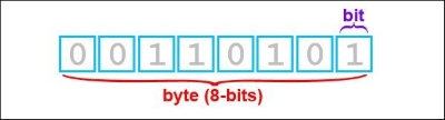
Each pixel in the previous topic has three channels: blue, green, and red. Each one has a value ranging from 0 to 255 (256 possible values). The combination of these channels result in a visible color. This range of values is not random; 256 is the number of combinations that is possible to achieve with a single byte.
A byte is the smallest portion of data that a computer can store and retrieve from the memory. It's composed of 8 bits of zeros or ones.
This is important to us because the computer uses its memory to store the image and it will reserve a given space to store the value for each channel for each pixel. We must be sure that the space reserved is adequate for the data we want to store.
Let's make an abstraction. Think that you have 1 liter (1,000 ml) of water and you want to store it. If you choose a 250 ml cup to store this water, the excess will spill out. If you choose a water truck with 10,000 liter capacity, you can store the water, but it will be a huge waste of space. So, you may choose a 3 liter bucket that would be sufficient to store the water. It's not big as a truck and you will have some extra space if you want to store a little bit more water.
In computing, things work similarly. You need to choose the size of the container before you put things in it. In the previous example, OpenCV made this choice for us. You will see a number of instances in the future where the programs we use will help us in these choices. But a clear understanding on how this works is very important because if the water spills out (that is, overflows), you will end up with unexpected behavior in your program. Or, if you choose a too large recipient, you may run out of computer memory.
The needs for value storage may vary in the aspects of:
- Only positive or positive and negative numbers
- Integers or fractions
- Small or large numbers
- Complex numbers
The available options and their sizes may vary with the computer architecture and software. For a common 64-bit desktop, NumPy will give you these possible numerical types:
bool: Boolean (True or False) stored as a byteint8: Byte (-128 to 127)int16: Integer (-32768 to 32767)int32: Integer (-2147483648 to 2147483647)int64: Integer (-9223372036854775808 to 9223372036854775807)uint8: Unsigned integer (0 to 255)uint16: Unsigned integer (0 to 65535)uint32: Unsigned integer (0 to 4294967295)uint64: Unsigned integer (0 to 18446744073709551615)float16: Half precision float: sign bit, 5 bits exponent, 10 bits mantissafloat32: Single precision float: sign bit, 8 bits exponent, 23 bits mantissafloat64: Double precision float: sign bit, 11 bits exponent, 52 bits mantissacomplex64: Complex number represented by two 32-bit floats (real and imaginary components)complex128: Complex number represented by two 64-bit floats (real and imaginary components)
So, we may expect that our sample image has the type uint8. Let's check whether it's true:
- Edit the
if __name__ == '__main__':block:if __name__ == '__main__': image = open_raster_file('../../data/sample_image.tiff') print(type(image)) print(image.dtype) - Run the code again. You should see an output matching our expectations:
<type 'numpy.ndarray'>
uint8

Process finished with exit code 0